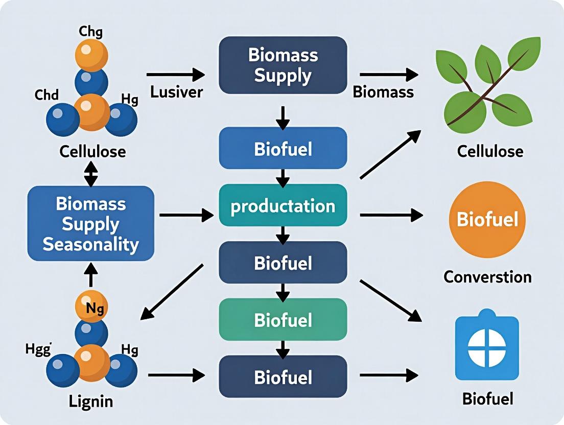
Strategies to Overcome Biomass Supply Seasonality in Sustainable Biofuel Production

Abstract

This article provides a comprehensive analysis of strategies to mitigate biomass supply seasonality, a critical bottleneck for consistent and cost-effective biofuel production. Targeting researchers and industry professionals, it explores the fundamental causes and impacts of seasonal variation (Intent 1), examines technical and logistical solutions for feedstock stabilization and storage (Intent 2), addresses common operational challenges and optimization techniques (Intent 3), and validates approaches through comparative analysis of lifecycle assessments and economic models (Intent 4). The synthesis offers a roadmap for developing resilient, year-round biomass supply chains essential for advancing biofuel technologies.

Understanding the Core Challenge: The Impact of Seasonal Biomass Variability on Biofuel Production

Technical Support Center: Troubleshooting Biomass Seasonality Experiments

FAQs & Troubleshooting Guides

Q1: Our pre-harvest biomass yield predictions for switchgrass are consistently overestimated by 15-20% compared to actual harvest data. What could be causing this discrepancy? A: This is a common calibration issue. The discrepancy often stems from using generic growth models that don't account for localized stress factors.

• Primary Check: Verify the soil moisture and precipitation data input into your model. A live search confirms that localized drought stress, even if short-term, can reduce final biomass yield significantly without affecting early-season growth metrics.
• Protocol Correction: Implement in-situ soil moisture sampling at the root zone (15-30 cm depth) bi-weekly for 8 weeks pre-harvest. Use a calibrated time-domain reflectometry (TDR) probe. Compare these readings to the regional weather station data used in your model.
• Solution: Recalibrate your yield prediction model with a site-specific drought stress coefficient derived from the TDR data.

Q2: When analyzing seasonal moisture content in miscanthus, we observe high variability within samples from the same harvest batch, compromising our dry ton calculations. How can we standardize sampling? A: Intra-batch variability indicates improper sub-sampling from heterogeneous biomass bales or stacks.

• Primary Check: Review your sub-sampling protocol. Grabbing material only from the outside of a bale will give higher moisture readings than from the core.
• Protocol Correction: Follow the standardized ASABE S358.3 method for forage and biomass moisture measurement.
  • Composite Sample: Use a core sampler to take a minimum of 5 cores from different locations and depths of at least 3 bales.
  • Immediate Processing: Coarsely chop and mix the composite sample in a sealed bag.
  • Rapid Sub-sampling: Quickly take three 100-150g sub-samples for triplicate analysis.
  • Drying: Dry in a forced-air oven at 105°C for 24 hours (or until constant mass) as per the standard.
• Solution: Implement this destructive composite sampling method. For non-destructive rapid screening, pair it with a calibrated NIR moisture meter, validating weekly against oven-dry results.

Q3: Our geospatial analysis for optimal biorefinery placement fails to accurately model winter biomass supply bottlenecks. What key seasonal factor are we likely missing? A: Your model likely uses annual average biomass productivity, missing Harvest Window Accessibility constrained by soil bearing capacity.

• Primary Check: Does your model incorporate soil type and monthly precipitation data to estimate field trafficability?
• Protocol Correction: Integrate a Soil Trafficability Index based on USDA Soil Survey Data and historical weather.
  • Data Layer Integration: Overlay biomass yield maps with soil type (especially clay content) and average monthly precipitation maps.
  • Index Calculation: For each 1km² grid, tag months where precipitation exceeds 90% of evapotranspiration + 20mm (saturated soil condition). These are "no-access" months for heavy harvesting equipment.
  • Supply Calculation: Model viable harvest months for each grid, shifting the available biomass to those periods.
• Solution: The bottleneck is not just growth, but harvestability. Include the trafficability index to identify regions where late-season harvests (post-senescence) are feasible versus those requiring early harvest with higher moisture.

Quantitative Data Summary

Table 1: Typical Seasonal Moisture Content & Yield Variation for Key Biofuel Feedstocks

Feedstock	Harvest Time	Avg. Moisture Content (% wet basis)	Estimated Dry Matter Yield (Mg/ha)	Key Geographical Consideration
Switchgrass	Post-Frost (Nov)	15-20%	8-12	Best in Midwestern US; delayed harvest reduces moisture but risks yield loss from lodging.
Miscanthus	Late Winter (Feb-Mar)	12-18%	14-20	Requires well-drained soils for winter access; not suitable for flood-prone areas.
Corn Stover	At Grain Harvest (Oct)	30-35%	3-5	Immediate collection required; high moisture necessitates drying or risk spoilage.
Sorghum	Physiological Maturity (Sep)	65-70%	10-15 (wet)	Grown in drier regions (e.g., Southern US); high moisture necessitates ensiling for storage.

Table 2: Impact of Pre-Harvest Factors on Biomass Quality

Factor	Measured Metric	Effect of Suboptimal Condition	Typical Range in Optimal Condition
Late-Spring Frost	Lignin Content	Increase of 2-4%	18-22% (switchgrass)
Summer Drought	Cellulose Crystallinity	Increase of 5-8%	45-55% (measured by XRD)
Excess Rainfall at Harvest	Ash Content	Increase of 1.5-3%	<5% (desired for thermochem. conversion)

Experimental Protocols

Protocol 1: Determining Region-Specific Harvest Windows Objective: To define the viable harvest period balancing yield maximization and moisture minimization for a given biomass crop and location. Methodology:

• Site Selection: Establish or identify three 0.25 ha replicate plots in the target region.
• Bi-weekly Sampling: Starting 2 weeks post-anthesis, collect 1m² of biomass from each plot every 2 weeks until spring regrowth.
• Measurements: For each sample, record (a) fresh weight, (b) dry weight (105°C oven), (c) stem count, and (d) visual lodging score.
• Soil Trafficability: Log daily precipitation. After any >10mm event, test soil bearing capacity with a penetrometer (reading >300 psi indicates equipment-safe).
• Analysis: Plot dry yield and moisture content over time. The viable harvest window is the period where dry yield plateaus, moisture is <25%, and soil bearing capacity is adequate.

Protocol 2: Standardized Moisture Content Correction for Supply Logs Objective: To provide a uniform method for reporting biomass deliveries on a dry ton basis. Methodology:

• Sample at Receival: As a truck is unloaded, take a minimum of 10 grab samples from the stream to form a ~5kg composite.
• Rapid Processing: Immediately coarse grind a 1kg subsample using a rotary mill.
• Drying: Weigh two ~100g aliquots of ground material (W_wet) into pre-weighed drying dishes. Dry at 105°C for 24 hours.
• Calculation: Weigh dried samples (Wdry). Moisture % = [(Wwet - Wdry) / Wwet] * 100. Dry Tonnage = Total Wet Tonnage * (100 - Avg. Moisture %) / 100.

Visualizations

Title: Decision Flow for Determining Biomass Harvest Window

Title: Core Strategies to Mitigate Biomass Supply Seasonality

The Scientist's Toolkit: Key Research Reagent Solutions

Table 3: Essential Materials for Biomass Seasonality Research

Item	Function in Research
Time-Domain Reflectometry (TDR) Probe	Measures real-time volumetric soil moisture content at various depths, critical for predicting harvest timing and plant stress.
Penetrometer	Measures soil compaction and bearing capacity to determine field accessibility for harvesting machinery during different seasons.
Forage/Core Sampler	Obtains representative cross-sectional samples from biomass bales or windrows for accurate moisture and composition analysis.
Forced-Air Drying Oven	Provides standardized drying at 105°C for determining the dry mass basis of biomass samples (the fundamental unit for supply calculations).
Portable NIR Spectrometer	Rapid, non-destructive field estimation of moisture and lignocellulosic composition when calibrated against primary methods.
Geographic Information System (GIS) Software	Integrates layers of yield data, soil type, climate, and infrastructure to model optimal harvest schedules and supply chains.
Weather Data Logger	Records localized microclimate conditions (precip, temp, humidity) at the field site, more accurate than distant station data.

Economic and Operational Consequences of Unstable Feedstock Supply

Technical Support Center: Troubleshooting Biomass Seasonality in Biofuel Research

FAQ & Troubleshooting Guide

Q1: Our pre-treatment efficiency for lignocellulosic biomass has dropped significantly with a new seasonal batch. How can we diagnose the issue? A: Seasonal variation in biomass composition (e.g., moisture, lignin, carbohydrate content) is the likely cause. Implement the following diagnostic protocol:

• Immediate Analysis: Perform proximate analysis (ASTM E871, E1755) and compositional analysis via NREL/TP-510-42618 method on the new batch.
• Comparative Data: Compare results with your baseline feedstock data in the table below.

Biomass Component	Baseline Batch (%)	New Seasonal Batch (%)	Tolerance Threshold (±%)
Moisture Content	12.5	28.7	3.0
Glucan	38.2	32.1	2.5
Xylan	23.1	19.8	2.0
Acid Insoluble Lignin	18.4	24.6	1.5
Ash	3.2	5.1	0.8

• Protocol - Adjusting Pre-treatment: If lignin or moisture exceeds thresholds, modify your dilute acid pre-treatment:
  • For High Moisture: Increase dry biomass loading by calculated mass to maintain consistent solid-to-liquid ratio.
  • For High Lignin: Increase pre-treatment severity (e.g., temperature by 5-10°C or residence time by 2-5 minutes). Always run a severity parameter (Log R₀) calculation to standardize.
  • Re-run compositional analysis on pre-treated solids to confirm consistent glucan recovery (>95% of baseline).

Q2: Our enzymatic hydrolysis yields are inconsistent due to feedstock variability. What is a robust experimental workflow to establish a correction factor? A: Follow this high-throughput screening protocol to generate a feedstock-specific response model.

Q3: Which signaling pathways in plant development are relevant to understanding biomass composition seasonality, and how can we model their impact? A: Key pathways affecting lignification and carbohydrate metabolism are central. The diagram below maps the relationship.

The Scientist's Toolkit: Key Research Reagent Solutions

Reagent/Material	Function in Mitigating Seasonality Studies	Example Vendor/Code
NREL Standardized Enzymatic Cocktail	Provides consistent, benchmarked hydrolytic activity for comparing biomass digestibility across variable samples.	NREL Cellic CTec3 / Sigma-Aldrich 71EMP
Monosaccharide Analysis Kit (HPLC)	Precisely quantifies glucose, xylose, etc., in hydrolysates for yield calculations.	Bio-Rad HPLC Carbohydrate Analysis Column
RNeasy Plant Mini Kit	Extracts high-quality RNA from diverse, seasonally harvested biomass for gene expression (qPCR) studies of lignification pathways.	Qiagen 74904
Lignin Quantification Kit	Rapid, spectrophotometric measurement of lignin content (acetyl bromide or thioglycolic acid method) for high-throughput screening.	Megazyme K-LIGNIN
Custom Synthetic Oligonucleotides	For qPCR primer design to monitor expression of key seasonality-responsive genes (e.g., PIFs, PAL, CesA).	Integrated DNA Technologies
Near-Infrared (NIR) Spectroscopy Calibration Set	For developing predictive models of biomass composition, enabling rapid screening of seasonal batches.	FOSS NIRSystems / Custom
Statistical Analysis Software	For multivariate regression of compositional data vs. process yields to establish robust correction factors.	JMP, R, or SIMCA

Technical Support Center: Troubleshooting Seasonal Biomass Supply Issues

Frequently Asked Questions (FAQs)

Q1: Our enzymatic hydrolysis yield of lignocellulosic biomass (e.g., corn stover) drops significantly when processing off-season (older, weathered) feedstocks. What is the primary cause and how can we mitigate it?

A1: The primary cause is the increase in lignin content and recalcitrance, and the loss of fermentable sugars due to environmental degradation during prolonged field storage. Mitigation strategies include:

• Pre-treatment Optimization: Increase severity (e.g., temperature, time) of your steam explosion or dilute acid pre-treatment for off-season batches. Conduct a quick compositional analysis (e.g., NREL LAP standards) to adjust parameters.
• Enzyme Cocktail Adjustment: Augment your cellulase mix with higher doses of β-glucosidase and lignin-degrading auxiliary enzymes (e.g., laccases).
• Additive Use: Include surfactants like Tween-80 or polyethylene glycol (PEG) to reduce non-productive enzyme binding to lignin.

Q2: We observe inconsistent lipid productivity in our open pond algal cultivation system with seasonal temperature and light variation. How can we stabilize yields?

A2: Inconsistency is expected due to photo-inhibition in summer and reduced metabolic rates in winter. Implement a robust monitoring and response protocol:

• Temperature: Use submerged temperature sensors. In summer, employ pulsed mixing or evaporative cooling. In winter, consider greenhouse covers or geothermal heat exchange if feasible.
• Light: Monitor PAR (Photosynthetically Active Radiation). In high-light seasons, operate at higher culture densities to self-shade cells and prevent photo-oxidation. Switch to strains with high light tolerance (e.g., Chlorella sorokiniana).
• Nutrient Stress Timing: Precisely control nitrogen deprivation triggers based on real-time cell density (optical density at 750 nm) rather than a fixed calendar schedule.

Q3: Our anaerobic digestion (AD) of food waste shows volatile fatty acid (VFA) accumulation and process inhibition during winter months, even in heated digesters. What's going wrong?

A3: This likely indicates thermal shock from feeding cold feedstock into a thermophilic digester, which stuns the microbial consortium. The problem is feed temperature, not just digester temperature.

• Solution: Pre-heat the waste slurry to within 5°C of the digester operating temperature (e.g., 55°C for thermophilic AD) before feeding. Implement a feed holding tank with simple heating.
• Monitoring: Increase VFA monitoring frequency (e.g., daily titrations or GC analysis) during seasonal transitions. If VFA:Alkalinity ratio exceeds 0.3, pause feeding and allow recovery.

Q4: How can we rapidly assess the quality of a new seasonal batch of biomass before committing to a full pre-treatment process?

A4: Implement a Two-Tier Analytical Protocol:

• Tier 1 (Rapid, <1 hr): Use Near-Infrared (NIR) spectroscopy calibrated for your biomass type to predict moisture, glucan, and lignin content.
• Tier 2 (Detailed, 1-2 days): Perform a modified Simons' Stain test to directly assess the accessible surface area of the biomass, which correlates well with enzymatic digestibility.

Troubleshooting Guides

Issue: Low Sugar Yield from Seasonal Lignocellulosic Feedstock

Symptom	Possible Cause	Diagnostic Test	Corrective Action
High solid residue post-hydrolysis	Increased lignin/ash content	Compositional Analysis (ASTM E1758)	Adjust pre-treatment severity; consider lignin-blocking additives.
Slow hydrolysis kinetics	Reduced pore volume from weathering	Simons' Stain (Cellulose Accessibility)	Increase biomass milling size reduction; optimize pre-treatment.
Microbial contamination in SSF	Higher native microbes in aged biomass	Agar plating of pre-hydrolysate	Apply a brief, mild disinfectant step (e.g., 1% H2O2 wash) pre-treatment.

Issue: Algal Culture Crash or Low Lipid Induction

Symptom	Possible Cause	Diagnostic Test	Corrective Action
Culture bleaching (summer)	Photo-oxidative damage	Chlorophyll Fluorescence (Fv/Fm)	Increase culture density; install shade cloths; reduce harvest rate.
Low growth rate (winter)	Suboptimal temperature	Daily biomass dry weight tracking	Switch to a cold-tolerant strain (e.g., Chlamydomonas nivalis); improve heating.
Poor nutrient uptake	Cold-induced metabolic slowdown	Nitrate/Phosphate assay in media	Pre-warm media; use readily available nitrogen sources (e.g., urea).

Experimental Protocols

Protocol 1: Modified Simons' Stain for Biomass Accessibility Objective: Quantify the accessible surface area of cellulose in a lignocellulosic biomass sample. Materials: Biomass sample (milled, 40-60 mesh), Direct Orange 15 (DO15, Pontamine Fast Scarlet), Direct Blue 1 (DB1, Pontamine Sky Blue), sodium citrate buffer (50 mM, pH 6.0), shaker, spectrophotometer. Procedure:

• Prepare separate 1 mM dye solutions of DO15 and DB1 in citrate buffer.
• Weigh 0.1g of biomass (triplicate) into centrifuge tubes.
• Add 10 mL of dye solution to each tube. For a full assay, run tubes with DO15 and DB1.
• Shake tubes at 60 RPM for 3 hours at room temperature.
• Centrifuge at 4000xg for 10 minutes.
• Dilute the supernatant 1:10 and measure absorbance (DO15 at 455 nm, DB1 at 624 nm).
• Calculate dye adsorbed (mg/g biomass) using calibration curves. The ratio of DO15/DB1 adsorbed correlates with digestibility.

Protocol 2: Rapid VFA:Alkalinity Ratio for AD Health Objective: Quickly assess imbalance in anaerobic digester. Materials: Digester slurry sample, 0.1N H2SO4, pH meter, magnetic stirrer, bromocresol green indicator. Procedure (Two-Point Titration):

• Filter 5 mL of slurry through a 0.45 µm filter.
• Dilute filtrate with 20 mL deionized water in a beaker.
• Place on stirrer, insert pH probe. Record initial pH.
• Titrate with 0.1N H2SO4 to pH 5.0. Record volume V1. This neutralizes bicarbonate alkalinity.
• Continue titrating to pH 4.4. Record total volume V2.
• Calculate: VFA as mg/L CH3COOH = (V2 * N * 60000) / Sample_Vol(5mL). Ratio = V2/(V2-V1). A ratio >0.3 indicates impending instability.

Pathway & Workflow Diagrams

Diagram Title: Seasonal Biomass Mitigation Workflow

Diagram Title: Anaerobic Digestion Cold Inhibition Pathway

The Scientist's Toolkit: Key Research Reagent Solutions

Reagent/Material	Primary Function	Application Notes
Pontamine Dyes (DO15 & DB1)	Stains cellulose to measure accessible surface area.	Critical for Simons' Stain assay. DO15 binds highly accessible cellulose, DB1 binds total.
Lignin-Blocking Surfactants (Tween-80, PEG 4000)	Reduces non-productive enzyme binding to lignin.	Add during enzymatic hydrolysis of weathered biomass to boost yield by 5-15%.
Fluorometric Chlorophyll Kits	Measures algal photosynthetic health via Fv/Fm.	Essential for detecting light stress in seasonal algal cultures. Target Fv/Fm > 0.6.
Specific VFA Standards (Acetic, Propionic, Butyric)	Calibration for GC analysis of AD intermediates.	Enables precise monitoring of digester health and early inhibition detection.
Custom Enzyme Cocktails (e.g., Cellic CTec3, HTec3)	Tailored blends of cellulases, hemicellulases, auxiliary activities.	Adjust ratio (e.g., more β-glucosidase) for degraded feedstocks.
Cold-Tolerant Algal Strains (e.g., UTEX 1663)	Engineered or wild-type strains for winter productivity.	Maintain culture collections with varied optimal temperatures.

The Role of Climate and Agronomic Practices in Feedstock Availability Fluctuations

Troubleshooting Guide & FAQ

Q1: Our lab’s enzymatic hydrolysis yield from seasonal switchgrass samples has dropped by 30% compared to the baseline. What could be the cause?

A: This is a common issue linked to feedstock compositional variability. Climate stress (e.g., drought) can increase lignin content and alter cellulose crystallinity. First, perform a compositional analysis (NREL/TP-510-42618) to compare the problematic batch with your baseline. A significant increase in acid-insoluble lignin (AIL) is the likely culprit.

Q2: We observe inconsistent biogas production from our anaerobic digestion of agricultural residues batch-to-batch. How can we stabilize the feedstock input?

A: Inconsistent methane yield often stems from variable volatile solids (VS) and carbon-to-nitrogen (C:N) ratio. Implement the following pre-processing protocol:

• Homogenize & Composite: Collect and grind residues from multiple field locations to create a composite sample.
• Pre-Treatment Assessment: Run a standard Biochemical Methane Potential (BMP) assay (see Protocol A below) on a subsample.
• Blending: Based on BMP and C:N results, blend different residue batches or add a co-substrate (e.g., manure) to achieve a C:N ratio between 20:1 and 30:1 before the main digester feed.

Q3: Cellulosic ethanol fermentation inhibitors (e.g., furfural, HMF) are spiking in our summer-harvested corn stover pre-hydrolysate. What agronomic or processing step can mitigate this?

A: High temperatures during the growing season can lead to higher pentosan concentrations, which degrade to furfural during pretreatment. Two mitigation strategies:

• Agronomic: Source stover from fields irrigated to avoid severe drought stress.
• Processing: Optimize your dilute-acid pretreatment severity. Reduce temperature or acid concentration, and implement an overliming step (adjusting hydrolysate to pH 10 with Ca(OH)₂, holding at 30°C for 1 hour, then re-neutralizing) to detoxify before fermentation.

Experimental Protocol A: Biochemical Methane Potential (BMP) Assay

Objective: To determine the ultimate methane yield of a seasonal biomass feedstock under anaerobic conditions.

Materials:

• Serum bottles (500 mL)
• Anaerobic inoculum (from an active digester)
• Substrate (seasonal biomass, ground to <1 mm)
• Positive control (microcrystalline cellulose)
• Negative control (inoculum only)
• Gas-tight syringes
• Anaerobic chamber (or gassing manifold with N₂/CO₂)
• BMP buffer medium (macro- and micronutrients)

Methodology:

• Prepare substrate bottles with a substrate-to-inoculum ratio of 0.5 gVS/gVS.
• Fill bottles with inoculum and BMP medium under anaerobic conditions.
• Flush headspace with N₂/CO₂ (70:30) for 2 minutes.
• Seal bottles and incubate at 35°C with continuous shaking.
• Monitor biogas production and composition (via GC-TCD) daily until production ceases.
• Calculate net methane yield from the substrate by subtracting the negative control yield.

Key Quantitative Data: Feedstock Variability

Table 1: Impact of Drought Stress on Key Biomass Compositional Parameters

Feedstock	Treatment	Cellulose (%TS)	Hemicellulose (%TS)	Lignin (%TS)	Ethanol Theoretical Yield (L/kg)
Switchgrass	Irrigated	38.2 ± 1.5	28.1 ± 0.9	18.5 ± 0.7	0.28 ± 0.01
Switchgrass	Drought-Stressed	32.7 ± 2.1	23.8 ± 1.3	25.4 ± 1.2	0.21 ± 0.02
Corn Stover	Normal Rainfall	37.9 ± 1.2	24.5 ± 1.0	16.8 ± 0.8	0.27 ± 0.01

Table 2: Effect of Harvest Timing on Biomass Yield and Quality

Feedstock	Harvest Date	Dry Matter Yield (Mg/ha)	Moisture Content (%)	Bulk Density (kg/m³)
Miscanthus	Early Fall	24.5 ± 2.1	55 ± 5	85 ± 10
Miscanthus	Late Winter	18.7 ± 1.8	15 ± 3	145 ± 15

Research Reagent Solutions & Essential Materials

Item	Function in Research
NREL Standard Biomass Analytical Protocols	Provides standardized methods for compositional analysis (e.g., Determining Structural Carbohydrates and Lignin).
Cellulolytic Enzyme Cocktail (e.g., CTec3)	Enzyme blend for hydrolyzing cellulose to fermentable sugars in saccharification assays.
Anaerobic Digestion Inoculum	Active microbial consortium from a stable biogas reactor, essential for BMP assays.
Microcrystalline Cellulose (Avicel PH-101)	Pure cellulose standard for positive controls in hydrolysis and fermentation experiments.
GC-TCD/FID System	For precise quantification of biogas (CH₄, CO₂) and fermentation inhibitors (furans, organic acids).
Near-Infrared (NIR) Spectrometer	For rapid, non-destructive prediction of biomass composition (calibration required).
Neutral Detergent Fiber (NDF) Assay Kit	For rapid fiber analysis to estimate cellulose/hemicellulose/lignin fractions.

Visualization: Feedstock Seasonality Mitigation Workflow

Title: Workflow for Mitigating Biomass Supply Seasonality

Visualization: Biomass Pre-Processing Decision Pathway

Title: Feedstock Quality Decision Tree for Pre-Processing

Practical Solutions: Feedstock Diversification, Storage, and Preprocessing Technologies

Technical Support Center: Troubleshooting & FAQs

This technical support center addresses common experimental challenges in multi-feedstock biomass research, framed within the thesis context of mitigating biomass supply seasonality for biofuel production.

Troubleshooting Guide: Common Experimental Issues

Issue 1: Inconsistent Saccharification Yields from Blended Feedstocks

• Symptoms: High variability in glucose release during enzymatic hydrolysis despite consistent pre-treatment.
• Root Cause: Inhomogeneous blending of feedstocks with different particle sizes and bulk densities (e.g., wheat straw vs. willow chips).
• Solution: Implement a standardized size-reduction and sieving protocol (e.g., all feedstocks milled to pass 2mm sieve) prior to gravimetric blending. Use a rotary drum blender for ≥30 minutes.

Issue 2: Inhibitor Buildup in Fermentation Broth

• Symptoms: Lag phase in fermentation, reduced ethanol/productivity, especially with forest product blends.
• Root Cause: Synergistic release of inhibitors (furfural, HMF, phenolic compounds) from lignin-rich blends during pre-treatment.
• Solution: Incorporate an over-liming or activated charcoal detoxification step post-hydrolysis. Monitor inhibitor concentrations via HPLC and adjust detoxification time accordingly.

Issue 3: Seasonal Variability in Composition of Agricultural Residue

• Symptoms: Statistical outliers in compositional analysis (e.g., lignin content) for the same residue type.
• Root Cause: Biomass harvested from different locations, seasons, or under different weather conditions.
• Solution: Source and create a large, homogenized batch of each feedstock. Characterize thoroughly (Table 1) and store under controlled conditions (15°C, <50% RH) for annual experiments.

Frequently Asked Questions (FAQs)

Q1: What is the optimal blending ratio for year-round biorefinery operation? A: There is no universal optimum. It depends on local feedstock availability and cost. The goal is to maintain a consistent, year-round supply of fermentable sugars. A dynamic blending model is required. See Table 2 for seasonal availability data to inform your model.

Q2: How do we pre-treat such heterogeneous blends effectively? A: Steam explosion and dilute acid pre-treatment show the most robustness for blended streams. However, a two-stage pre-treatment may be necessary if feedstocks have highly divergent recalcitrance (e.g., softwood with grasses). Always perform a compositional analysis after blending to calibrate pre-treatment severity.

Q3: Our enzymatic hydrolysis efficiency drops when we include more than 20% forest residues. Why? A: Forest residues, especially from softwoods, have higher lignin and acetyl content, which non-productively bind cellulases. Solution: 1) Increase enzyme loading proportionally, or 2) Supplement with lignin-blocking additives (e.g., bovine serum albumin or Tween-80), or 3) Consider a milder pre-treatment on the forest stream separately before blending.

Q4: How should we store seasonal feedstocks to minimize degradation? A: Dry agricultural residues to <10% moisture content and pelletize for dense, stable storage. Energy crops like switchgrass can be ensiled anaerobically. Forest products should be chipped and kept under cover to prevent leaching. Monitor for dry matter loss.

Data Presentation

Table 1: Typical Compositional Range of Primary Feedstock Categories (Dry Basis %)

Feedstock Category	Cellulose	Hemicellulose	Lignin	Ash	Notes
Agricultural Residue (e.g., Corn Stover)	35-40	20-25	15-20	4-8	High seasonal variability; ash can be high.
Herbaceous Energy Crops (e.g., Switchgrass)	32-37	25-30	15-20	3-6	More consistent; harvestable in fall.
Short-Rotation Woody Crops (e.g., Willow)	40-45	20-25	22-27	0.5-2	Low ash; high lignin; harvestable in winter.
Forest Residues (e.g., Pine Thinnings)	40-45	20-23	26-30	<1	Highest lignin; very stable supply.

Table 2: Illustrative Seasonal Availability Index for North American Feedstocks

Feedstock	Q1 (Jan-Mar)	Q2 (Apr-Jun)	Q3 (Jul-Sep)	Q4 (Oct-Dec)	Supply Risk Factor*
Corn Stover	Low (10)	Low (10)	Medium (40)	High (100)	High (Weather-dependent)
Wheat Straw	Medium (50)	Low (20)	Low (10)	High (100)	High (Weather-dependent)
Switchgrass	Low (30)	Medium (60)	High (90)	High (100)	Medium (Established stand)
Willow	High (100)	Medium (50)	Low (20)	High (100)	Low (Storage possible)
Forest Residues	High (100)	High (100)	High (100)	High (100)	Very Low (Year-round)

Scale: 0-100, where 100 = peak harvest/availability. *Supply Risk Factor: Likelihood of shortage due to harvest conditions.

Experimental Protocols

Protocol 1: Standardized Feedstock Blending and Compositional Analysis Objective: To create a homogeneous, characterized blended feedstock for seasonal simulation experiments. Methodology:

• Preparation: Separately mill individual feedstocks to pass a 2mm sieve. Dry at 45°C to constant weight.
• Gravimetric Blending: Calculate masses needed for target dry-weight ratio (e.g., 40% stover, 30% switchgrass, 30% willow). Use an analytical balance.
• Homogenization: Combine masses in a rotary drum blender for 45 minutes.
• Compositional Analysis: Perform triplicate analysis of the blend using NREL/TP-510-42618 standard procedures for determination of structural carbohydrates and lignin.
• Storage: Store homogenized blend in airtight containers with desiccant at 4°C.

Protocol 2: Two-Stage Pre-treatment for High-Lignin Blends Objective: To improve sugar recovery from blends containing >25% forest products. Methodology:

• Separation: Separate the blended feedstock into a "high-lignin" fraction (forest products) and "low-lignin" fraction (residues/crops).
• Stage 1 (High-Lignin Fraction): Apply a mild alkaline pre-treatment (e.g., 1% NaOH, 120°C, 60 min). Wash solid fraction.
• Stage 2 (Combined Stream): Recombine the pre-treated high-lignin solids with the raw low-lignin fraction.
• Main Pre-treatment: Apply standard dilute-acid steam explosion (e.g., 1% H2SO4, 180°C, 15 min) to the recombined slurry.
• Analysis: Neutralize hydrolysate, filter, and analyze for monomeric sugars and inhibitors via HPLC. Compare yield to single-stage pre-treatment.

Mandatory Visualizations

Diagram Title: Multi-Feedstock Strategy for Mitigating Seasonality

Diagram Title: Experimental Workflow for Blended Feedstock Processing

The Scientist's Toolkit: Research Reagent Solutions

Item	Function / Application	Key Consideration
Cellulase Enzyme Cocktail (e.g., CTec3)	Hydrolyzes cellulose to glucose.	Loading must be optimized for blend lignin content.
Lignin-Blocking Additive (e.g., BSA, Tween-80)	Reduces non-productive enzyme binding to lignin.	Critical for blends with high forest product content.
Internal Standard for HPLC (e.g., Erythritol)	Quantifies sugar and inhibitor concentration in hydrolysate.	Must not interfere with analyte peaks.
NREL Standard Analytical Procedures	Provides rigorous, comparable compositional data.	Essential for publication-quality data.
Anaerobic Chamber / Sealed Vials	For simulating industrial-scale fermentation conditions.	Ensures reproducibility in inhibition studies.
Customized Blending Software / Spreadsheet Model	Calculates dynamic blending ratios based on cost & availability.	Core tool for translating research to operational strategy.

Technical Support Center: Troubleshooting & FAQs

FAQ Section

Q1: In our ensiling trials for switchgrass, we observe pH stagnation around 5.2 instead of dropping below 4.8, leading to spoilage. What are the primary causes and corrective actions? A: pH stagnation typically indicates insufficient lactic acid fermentation. Common causes and solutions are:

• Low Water-Soluble Carbohydrate (WSC) Content: Ensure biomass is harvested at the optimal maturity stage (e.g., boot stage for grasses). Consider applying a biological inoculant containing homofermentative Lactobacillus strains (e.g., L. plantarum, L. buchneri) at 1 x 10^5 CFU per gram of fresh material to efficiently convert available sugars to lactic acid.
• Excessive Dry Matter (DM): If DM >50%, microbial activity is limited. The target DM for optimal ensiling is 30-45%. Use a moisture meter at harvest and consider wilting or adding water as needed.
• Inadequate Compaction: Poor compaction leaves excess oxygen, promoting yeast and mold growth. Use standardized packing density protocols (target >220 kg DM/m³). Re-open the silo, re-chop to a shorter theoretical length of cut (10-15 mm), and repack immediately.

Q2: During controlled atmosphere storage of woody biomass (e.g., poplar chips), we detect elevated CO levels (>100 ppm) despite maintaining low O2 (0.5-1.0%). Is this a sign of hazardous fermentation or normal respiration? A: Elevated CO is a critical safety and quality warning. While trace CO can be produced from lipid oxidation, levels >50 ppm often indicate incipient spontaneous heating. This is not normal respiration.

• Immediate Action: Cease entry into the storage facility. Ventilate with air to increase O2 levels to >5% temporarily to break the exothermic reaction chain.
• Corrective Protocol: Re-analyze the biomass moisture content. For CA storage of chips, moisture must be kept below 25% (wet basis). Check sensor calibration for O2 and temperature. Introduce a stepped aeration cycle (4 hours on, 8 hours off) until the temperature stabilizes at <5°C above ambient.

Q3: When analyzing dry matter losses (DML) in our silage samples, we find discrepancies between oven drying (105°C) and Near-Infrared Spectroscopy (NIRS) methods. Which is the definitive standard for biofuel feedstock quality analysis? A: For definitive chemical composition data (e.g., cellulose, hemicellulose, lignin) required for conversion yield calculations, the oven drying method (105°C to constant weight) followed by sequential detergent fiber analysis (e.g., Van Soest method) is the required standard. NIRS is a rapid, non-destructive tool for in-situ quality monitoring but must be calibrated against wet chemistry data from your specific biomass type and storage conditions. Re-calibrate your NIRS model using at least 50 representative calibration samples that have been analyzed via the standard oven-drying and wet chemistry protocols.

Q4: Our biomass exhibits significant sugar degradation after 6 months of hermetic bag storage. How do we differentiate between enzymatic hydrolysis and microbial consumption? A: This requires targeted metabolite and microbial community analysis.

• Protocol to Diagnose:
  • Sample: Aseptically collect material from the core.
  • Extract & Analyze: Perform aqueous extraction and analyze via HPLC for organic acids (lactic, acetic, butyric), ethanol, and residual sugars (glucose, xylose, fructose).
  • Interpretation: High acids/ethanol with low sugars indicate microbial consumption. High levels of oligomeric sugars (requires enzymatic hydrolysis post-extraction for detection) with low acids suggest ongoing enzymatic hydrolysis from native plant enzymes.
  • Solution: For future batches, consider a fast-acting acid-based additive (e.g., formic acid at 2-3 L/t) to immediately lower pH and inhibit both plant enzymes and microbes.

Troubleshooting Tables

Table 1: Common Ensiling Issues & Solutions

Symptom	Probable Cause	Diagnostic Test	Corrective Action
Surface Mold & Heating	Oxygen infiltration, poor sealing	Check plastic for holes; measure temperature profile	Apply an oxygen barrier film; increase packing density; use L. buchneri inoculant.
Clostridial Spoilage (Butyric smell, high NH3-N)	Wet material (>70% moisture), low WSC	Analyze for butyric acid, ammonia-N content	Wilt to >30% DM; ensure rapid initial pH drop with inoculant.
Effluent Production	DM too low (<25%)	Weigh storage bunker/bag periodically for loss	Add absorbents (e.g., dried beet pulp, straw) at ensiling; pre-wilt.

Table 2: Controlled Atmosphere Storage Parameters for Bioenergy Feedstocks

Biomass Type	Recommended O2 (%)	Recommended CO2 (%)	Temperature Max (°C)	Target Moisture (% wet basis)	Max Storage Duration (months)
Corn Stover Bales	<1.0	>20	35	15-20	12
Miscanthus Chips	0.5 - 1.5	15-25	40	18-25	9
Poplar/Woody Chips	1.0 - 2.0	10-20	35	20-25	12
Wheat Straw	<1.5	>15	30	12-15	15

Experimental Protocol: Evaluating Additives for Dry Matter Preservation

Objective: To quantify the efficacy of chemical vs. biological additives in preserving fermentable sugars in grass biomass during storage.

Materials:

• Freshly harvested biomass (e.g., perennial ryegrass).
• Treatments: a) Control (deionized water), b) Homolactic inoculant (e.g., L. plantarum), c) Heterolactic inoculant (e.g., L. buchneri), d) Chemical additive (e.g., potassium sorbate + sodium benzoate solution).
• Laboratory-scale silos (mini-silos, e.g., 1.5L vacuum bags or PVC pipes with sealed lids).
• pH meter, forced-air oven, HPLC system, mortar and pestle, liquid nitrogen.

Methodology:

• Preparation: Chop biomass to 10-20 mm. Determine initial DM and WSC content.
• Application: Apply treatments evenly via a hand sprayer to achieve 5 mL per kg of fresh material. For control, apply an equal volume of water.
• Ensiling: Pack treated biomass tightly into triplicate mini-silos per treatment. Remove air by vacuum sealing or physical compression and sealing. Store at ambient temperature (20-25°C).
• Sampling: Open silos after 0, 7, 30, and 90 days.
• Analysis:
  • pH: Measure in a water extract (10g sample in 90mL DI water).
  • DM Loss: Weigh silo contents before and after, correcting for DM.
  • Metabolite Profile: Freeze-dry a sub-sample, grind, and extract sugars and acids for HPLC analysis.
  • Fibre Composition: Perform Neutral Detergent Fiber (NDF) and Acid Detergent Fiber (ADF) analysis on dried samples.

Visualization: Experimental Workflow for Biomass Storage Trials

Title: Biomass Storage Experiment Workflow

The Scientist's Toolkit: Key Research Reagent Solutions

Table 3: Essential Materials for Biomass Storage Research

Item	Function/Application	Key Consideration for Research
Homofermentative Inoculant (e.g., Lactobacillus plantarum)	Drives rapid pH drop in silage via efficient lactic acid production.	Ensure strain specificity and CFU count (>1x10^10/g); use for high-WSC biomass.
Heterofermentative Inoculant (e.g., Lactobacillus buchneri)	Produces acetic acid, improving aerobic stability at feed-out.	Apply for biomass prone to spoilage upon exposure to air; slower initial fermentation.
Chemical Preservative (e.g., Formic Acid, Sodium Benzoate)	Directly acidifies or inhibits spoilage microbes independent of fermentation.	Use for low-WSC biomass; corrosive; requires precise dosing equipment.
Oxygen Barrier Film (e.g., multi-layer polyethylene with EVOH)	Minimizes oxygen permeability in bunkers, bags, or bale wraps.	Critical for controlled atmosphere experiments; standard plastic is insufficient.
Gas Analyzer (O2/CO2/CO/CH4)	Monitors atmosphere composition in real-time during CA storage.	Must have low detection limits (<0.1% for O2/CO2) and be calibrated regularly.
Anaerobe Bag System	Creates anaerobic environment for small-scale ensiling studies (mini-silos).	Provides standardized, replicable conditions for treatment comparisons.
Neutral & Acid Detergent Solutions (for NDF/ADF analysis)	Quantifies fiber components (cellulose, hemicellulose, lignin) to assess quality.	The standard Van Soest method is essential for correlating storage losses to convertible sugars.
Cryogenic Grinder (e.g., with liquid nitrogen)	Homogenizes fibrous biomass for representative sub-sampling for chemical analysis.	Essential for obtaining accurate, replicable data from heterogeneous stored material.

Technical Support Center

Troubleshooting Guides & FAQs

1. Feedstock Preprocessing & Densification

• Q1: Our pellet mill is experiencing severe die blockage and producing excessively fractured pellets. What are the likely causes and solutions?

  • A: This typically indicates improper feedstock conditioning.
    • Cause 1: Incorrect Moisture Content. Biomass moisture is outside the optimal range of 8-12% (for wood) for densification.
    • Solution: Implement a pre-drying step (e.g., rotary drum dryer) and install an online moisture sensor for real-time feedback to the dryer control system.
    • Cause 2: Inconsistent Particle Size. A wide distribution of particle sizes leads to poor interlocking and binding.
    • Solution: Incorporate a two-stage grinding (shredder followed by hammer mill) and sieving system to ensure 95% of feedstock is within 1-4 mm.
    • Cause 3: Lack of Natural Binders. Some herbaceous biomass (e.g., straw) has low lignin content.
    • Solution: Use a starch-based binder (e.g., 1-3% by weight) or adjust process temperature to slightly melt lignins.

• Q2: How do we quantitatively assess the durability and storage stability of produced pellets/briquettes?

  • A: Follow the standardized protocol below.
    • Protocol: Pellet Durability & Hygroscopicity Test.
      • Durability Index (DI): Place 500 g of pellets (Pinitial) in a standard tumbler (e.g., ASAE S269.5). Rotate at 50 rpm for 10 minutes.
      • Sieve to remove fines (particles < 3.15 mm). Weigh the remaining pellets (Pfinal).
      • Calculate: DI (%) = (Pfinal / Pinitial) * 100. Target: >97.5% for commercial-grade.
      • Hygroscopicity: Place pre-weighed (W_initial), oven-dried pellets in a climate chamber at 30°C and 90% RH for 48 hours.
      • Weigh again (Wfinal). Calculate moisture uptake: ΔM (%) = [(Wfinal - Winitial) / Winitial] * 100.

Quantitative Data Summary: Pellet Quality Metrics

Feedstock Type	Optimal Moisture Content (%)	Optimal Die Temp. (°C)	Typical Durability Index (%)	Hygroscopicity ΔM (48h, 90% RH) (%)
Pine Sawdust	8-10	90-110	98.2-99.5	3.1-4.5
Wheat Straw	10-12	70-90	94.5-97.0	7.8-10.2
Torrefied Wood	5-7	70-80	99.0-99.8	1.5-2.5

2. Torrefaction Reactor Operation

• Q3: Our torrefied biomass shows inconsistent properties (energy density, grindability) between batches. How do we stabilize the process?

  • A: Inconsistency stems from poor control of the "3Ts": Temperature, Time, and atmosphere.
    • Step 1: Calibrate Sensors. Verify and calibrate thermocouples (at multiple reactor bed locations) and inert gas (N2) flow meters monthly.
    • Step 2: Standardize Protocol. Adhere to a strict experimental matrix. Example:
      • Protocol: Fixed-Bed Torrefaction.
        • Load 200 g of dried, pelletized biomass into the reactor.
        • Purge with N2 at 5 L/min for 15 minutes to achieve O2 < 2%.
        • Heat at 10°C/min to target torrefaction temperature (e.g., 250, 275, 300°C).
        • Maintain (Residence Time) for 30 minutes under continuous N2 flow (2 L/min).
        • Cool to <50°C under N2 before unloading.
    • Step 3: Monitor Output. Calculate Mass Yield (MY) = (Mfinal / Minitial) * 100 and Energy Yield (EY) = MY * (HHVfinal / HHVinitial) for every batch. A deviation >±2% from the expected value indicates a process variable drift.

• Q4: What are the main safety risks with torrefaction off-gases, and how are they managed?

  • A: Off-gases (torr-gas) are flammable (CO, CH4) and contain condensable acids (formic, acetic).
    • Risk 1: Explosion. Ensure the reactor headspace is always under inert atmosphere during heating/cooling.
    • Solution: Install a flame arrester and a pressure relief valve on the gas outlet line. Maintain N2 purge until reactor is cold.
    • Risk 2: Corrosion. Condensable acids can damage piping and condensers.
    • Solution: Use stainless steel (316L) or PTFE for all wetted parts. Install a cold trap (maintained at -10 to 0°C) followed by a caustic scrubber (NaOH solution, pH >10) to capture condensables.

3. Fast Pyrolysis for Bio-Oil

• Q5: Our fast pyrolysis bio-oil is rapidly aging—increasing in viscosity and phase separating within days. What stabilization strategies can we apply immediately post-production?

  • A: Aging is caused by reactive aldehydes, ketones, and acids. Apply post-condensation stabilization.
    • Strategy 1: Hot Vapor Filtration. Pass pyrolysis vapors through a high-temperature (400-500°C) ceramic or sintered metal filter (pore size 0.5-2 µm) before condensation to remove alkali metals and char particles that catalyze polymerization.
    • Strategy 2: Solvent Addition. Immediately upon collection, blend bio-oil with a stabilizing solvent. Common reagents:
      • Methanol (10-20 wt%): Acts as a hydrogen donor, reduces viscosity, inhibits polymerization.
      • Ethanol (10-15 wt%): Similar effect, with higher biogenic carbon content.
      • Acetone (5-10 wt%): Improves homogeneity and lowers aging rate.
    • Protocol: Accelerated Aging Test. To compare stabilization efficacy, store oil samples at 80°C for 24h. Measure viscosity increase every 6h using a micro-viscometer. A well-stabilized oil should show <50% viscosity increase under this test.

• Q6: How do we troubleshoot blockages in the fast pyrolysis vapor quenching and condensation system?

  • A: Blockages are typically due to heavy ends condensing in transfer lines.
    • Symptom: Pressure increase upstream of condenser.
      • Immediate Action: Switch vapor flow to a standby condenser if available. Isolate and heat the blocked line with traced heating tape to 60-80°C to re-vaporize heavy condensates.
      • Preventive Redesign:
        • Minimize Dead Zones: Use swept-tee fittings and avoid sharp bends.
        • Increase Temperature: Maintain all vapor transfer lines >400°C until the quenching zone.
        • Optimize Quench: Use a direct-contact spray of cold, stabilized bio-oil or a low-boiling-point solvent (e.g., acetone) instead of a static shell-and-tube condenser for rapid quenching.

Quantitative Data Summary: Fast Pyrolysis Bio-Oil Stabilization

Stabilization Method	Initial Viscosity (cP, 40°C)	Viscosity Increase after 80°C/24h Test (%)	Water Content Change (absolute %, wt)
None (Raw Oil)	120-180	150-400	+0.5
10 wt% Methanol Addition	55-80	25-40	+2.0
Hot Vapor Filtration	90-140	80-120	-0.2
Combined (Filtration + 10% MeOH)	50-75	10-25	+1.8

The Scientist's Toolkit: Research Reagent Solutions

Item	Function & Rationale
Lignin-based Binder (e.g., Sodium Lignosulfonate)	Added during pelletizing (1-5% wt) to enhance binding for low-lignin feedstocks, improving mechanical durability.
Inert Gas (High-Purity N2, >99.999%)	Creates an oxygen-free environment for torrefaction and pyrolysis, preventing combustion and controlling reaction pathways.
Silicon Oil (for Fluidized Bed)	Acts as a high-temperature (up to 500°C) heat transfer medium in fluidized bed pyrolysis reactors for uniform heating.
Quenching Solvent (HPLC Grade Methanol)	Rapidly condenses pyrolysis vapors when sprayed directly, minimizing secondary cracking; also used for bio-oil stabilization.
Ceramic Filter Element (0.5 µm pore, 400°C rated)	Removes catalytic char and ash particles from hot pyrolysis vapor, reducing bio-oil aging rate.
Dehydration Catalyst (ZSM-5 Zeolite Powder)	Used in catalytic fast pyrolysis experiments to promote deoxygenation reactions, increasing hydrocarbon yield in bio-oil.
Internal Standard for GC-MS (e.g., Fluoranthene-d10)	Added to bio-oil samples before analysis to enable quantitative determination of compound concentrations via Gas Chromatography.
Stabilizer Cocktail (BHT + TPP)	Butylated Hydroxytoluene (antioxidant) and Triphenyl Phosphite (acid scavenger) added in ppm levels to inhibit polymerization.

Experimental Workflow Diagram

Title: Biomass Preprocessing Pathways & Troubleshooting Points

Bio-Oil Aging & Stabilization Pathways

Title: Bio-Oil Degradation Pathways and Stabilization Interventions

Logistical Modeling for Optimal Harvest Schedules and Supply Chain Network Design

Technical Support Center

Frequently Asked Questions (FAQs)

Q1: My biomass quality simulation model is showing high variance in moisture content predictions, leading to unreliable harvest schedule optimization. What could be the cause? A: High variance often stems from insufficient temporal resolution in weather data integration or incorrect degradation kinetics parameters. Ensure you are using hourly precipitation and humidity data instead of daily averages. Re-calibrate the moisture adsorption/desorption model using the standard protocol below (Protocol 1).

Q2: When designing a multi-feedstock supply chain network, my Mixed-Integer Linear Programming (MILP) solver fails to find a feasible solution. How should I troubleshoot? A: Infeasibility in this context typically originates from over-constrained storage capacity parameters or unrealistic transportation distance constraints. First, relax all storage capacity constraints and incrementally tighten them to identify the bottleneck. Verify that the distance matrix between potential depot locations and processing facilities is logically consistent.

Q3: My geospatial analysis for optimal harvest zone selection yields discontinuous, patchy zones that are logistically impractical. How can I rectify this? A: This is a common issue when using raw biomass yield potential as the sole criterion. You must incorporate a spatial clustering penalty or a contiguity constraint into your objective function. Apply a kernel-based smoothing function to the raw yield map before running the location-allocation algorithm.

Q4: The "seasonality mitigation index" calculated from my model does not align with observed historical biomass availability data. What parameters are most sensitive? A: The index is highly sensitive to the assumed storage degradation rate and the contractual flexibility percentage with suppliers. A 10% error in the degradation rate coefficient can lead to a >30% deviation in the index. Follow Protocol 2 for accurate degradation rate calibration.

Q5: How do I validate the robustness of my optimal harvest schedule against unexpected weather disruptions? A: Implement a Monte Carlo simulation framework where key weather variables (e.g., rainy days) are drawn from historical distributions. Run your scheduling model through 1000+ iterations to generate a distribution of possible outcomes and identify schedule fragility points. The resilience score can be calculated as shown in Table 2.

Detailed Troubleshooting Guides

Issue: Inaccurate Biomass Degradation Modeling in Storage. Symptoms: Predicted dry matter loss (DML) is consistently 15-20% lower than empirically measured loss in pilot-scale storage piles. Diagnosis Steps:

• Check the form of the degradation equation. The simple exponential decay model is often inadequate.
• Verify the temperature and moisture coupling function in your model. Most open-source models use an outdated multiplicative approach.
• Confirm the initial quality data (particle size, compaction) of biomass entering storage. Solution: Switch to a coupled discrete-continuous model that separates microbial heating phases from abiotic degradation. Integrate real-time temperature sensor data (from IoT devices) for dynamic model updating. Use the parameters in Table 1 for common feedstocks.

Issue: Supply Chain Network Model Performance Degradation with Increased Node Count. Symptoms: Solver time increases exponentially when modeling more than 50 potential depot locations. Diagnosis Steps:

• Profile your code to identify if the bottleneck is in matrix construction or the solver itself.
• Check the sparsity of your distance/ cost matrix. Solution: Implement a Benders Decomposition or a heuristic pre-processing step (e.g., p-median clustering) to reduce the problem size. Use commercial solvers like Gurobi or CPLEX which have advanced presolve capabilities for large-scale MILP.

Experimental Protocols

Protocol 1: Calibration of Biomass Moisture Content (MC) Prediction Model Objective: To empirically determine parameters for the MC adsorption/desorption model. Materials: See "Research Reagent Solutions" table. Method:

• Prepare 20 samples of comminuted feedstock (e.g., miscanthus, switchgrass).
• Place samples in controlled climate chambers at 5 distinct temperature (T) and relative humidity (RH) setpoints replicating harvest season conditions.
• Weigh samples using a precision balance (±0.01g) at t=0, 1, 2, 4, 8, 24, 48 hours.
• Dry a subset of samples at 105°C for 24h after each weighing to determine actual MC.
• Fit the data to the modified Henderson model: MC = a - ln(1-RH) / (b*T)^c using non-linear least squares regression.
• Validate fitted parameters against a hold-out dataset.

Protocol 2: Determination of Storage Dry Matter Loss (DML) Kinetics Objective: To quantify dry matter loss over time for key feedstocks under covered and uncovered storage. Materials: Pilot-scale storage bunkers (5m x 5m x 3m), temperature probes, moisture probes, tarpaulin covers, representative biomass bales. Method:

• Instrument three replicate storage piles per feedstock per condition (covered/uncovered) with a sensor grid.
• Record core temperature and ambient conditions daily.
• At days 0, 30, 90, 180, and 270, conduct core sampling using a hollow auger from 5 pre-determined locations per pile.
• Analyze samples for dry matter (DM), compositional sugars, and ash content via NREL standard laboratory analytical procedures.
• Model DML using a first-order kinetic reaction with an Arrhenius-type dependence on temperature: d(DML)/dt = A * exp(-Ea/(R*T)).

Data Presentation

Table 1: Calibrated Model Parameters for Biomass Degradation Kinetics

Feedstock	Storage Type	Pre-exponential Factor (A) [day⁻¹]	Activation Energy (Ea) [kJ/mol]	Dry Matter Loss at 180 days (%)
Switchgrass	Covered Pile	5.2 x 10⁵	55.2	12.4 ± 1.8
Switchgrass	Uncovered	8.9 x 10⁵	52.1	22.7 ± 3.1
Corn Stover	Baled & Wrapped	3.1 x 10⁵	58.7	8.5 ± 1.2
Corn Stover	Open Bale	7.4 x 10⁵	53.8	31.5 ± 4.5
Poplar Chips	Enclosed Silo	1.8 x 10⁵	61.3	6.3 ± 0.9

Table 2: Supply Chain Resilience Metrics Under Stochastic Disruption (Monte Carlo Simulation, n=5000)

Network Configuration	Avg. Cost Increase (%)	95th Percentile Cost Increase (%)	Seasonality Mitigation Index (SMI)	Probability of Critical Shortfall (<85% demand)
Centralized Depot (1)	34.7	89.2	0.45	0.18
Regional Depots (3)	18.1	41.5	0.72	0.05
Distributed Nodes (5+)	12.3	29.8	0.88	0.02

Diagrams

Title: Biomass Harvest Schedule Optimization Workflow

Title: Biofuel Supply Chain Network Structure

The Scientist's Toolkit: Research Reagent Solutions

Item	Function in Experiment	Key Specification/Note
Controlled Climate Chamber	Simulates field conditions for moisture adsorption/desorption studies.	Must control Temp. (±0.5°C) and RH (±2%) independently.
Precision Balance	Measures minute changes in biomass sample weight for MC calculation.	Required resolution: ±0.01g; with environmental chamber.
Hollow Core Auger	Extracts representative samples from deep within storage piles for DML analysis.	Stainless steel, length >3m, internal sample retention.
Wireless Temperature/Moisture Probe Grid	Logs real-time spatial data from biomass storage piles for model calibration.	IP67 rating, 30+ day battery, mesh network capable.
Geographic Information System (GIS) Software	Analyzes spatial yield data, transportation routes, and optimal depot placement.	Must support raster algebra and network analysis toolkits.
Mathematical Programming Solver	Solves large-scale optimization models (MILP, NLP) for scheduling and network design.	Gurobi, CPLEX, or COIN-OR CBC with Python/AMPL API.
Biomass Composition Analyzer	Quantifies structural carbohydrates, lignin, and ash for quality tracking.	Uses NREL/TP-510-42618 standard methods.

Overcoming Hurdles: Managing Degradation, Costs, and Supply Chain Disruptions

Technical Support Center: Troubleshooting & FAQs

This support center provides solutions for common experimental challenges in biomass storage research, framed within the thesis context of Mitigating biomass supply seasonality in biofuel production.

Troubleshooting Guide: Common Storage Experiment Issues

Q1: We are observing unexpectedly high dry matter loss (>25%) in our ensiled corn stover after 60 days, despite achieving an initial target pH of 4.2. What could be the cause? A1: High dry matter loss post-stabilization often indicates secondary clostridial fermentation or aerobic spoilage.

• Check 1: Measure Volatile Fatty Acid (VFA) profile. A high butyric acid concentration (>0.1% of fresh weight) confirms clostridial activity, often due to low water-soluble carbohydrate (WSC) content or high buffering capacity in the initial biomass.
• Check 2: Inspect storage integrity. Seal leaks can cause aerobic spoilage. Use an infrared gas analyzer to check for CO2 plume leaks.
• Protocol - VFA Analysis: Homogenize 20g of silage with 180ml of deionized water for 3 min. Filter through Whatman No. 54 paper. Analyze filtrate using High-Performance Liquid Chromatography (HPLC) with an Aminex HPX-87H column (Bio-Rad) at 45°C, using 5mM H2SO4 as mobile phase at 0.6 ml/min. Detect using a refractive index detector.

Q2: Our spectroscopic analysis (NIR) for predicting biomass quality shows poor calibration (R² < 0.80) when applied to new harvest batches. How can we improve model robustness? A2: This is a classic case of model overfitting or insufficient spectral library diversity.

• Action 1: Expand calibration set. Include samples from multiple harvest years, geographic locations, and pretreatment conditions (particle size, moisture gradients) to capture natural variability.
• Action 2: Apply standard normal variate (SNV) and detrending scatter corrections to NIR spectra to minimize physical light-scattering effects.
• Protocol - Robust NIR Calibration: Scan ≥150 representative samples in triplicate using a Fourier Transform NIR spectrometer (10,000–4,000 cm⁻¹ resolution: 8 cm⁻¹). Reference values for calibration must be obtained via standard wet chemistry (e.g., ANSI/ASAE S358.3 for moisture). Use partial least squares regression (PLSR) with full cross-validation.

Q3: During laboratory-scale aerobic storage of wood chips, the temperature exceeds the safe threshold of 65°C, risking spontaneous combustion. What immediate and preventive measures are required? A3: This indicates excessive microbial respiration or exothermic oxidation.

• Immediate Action: Disassemble the pile in a fume hood to promote cooling. Do not add water, as it can exacerbate microbial activity.
• Preventive Protocol: Monitor O2 concentration in the pile headspace. Maintain bulk density > 250 kg/m³ for chips to limit air infiltration. Implement a forced aeration system with a feedback loop: when internal temp > 55°C, blow ambient air at 0.05 m³/min per m³ of biomass.

Q4: When testing novel biological preservatives (e.g., Lactobacillus buchneri), how do we definitively attribute improved stability to the additive and not native microflora? A4: Use a combination of selective plating and molecular tracking.

• Protocol - Additive Efficacy:
  • Sample Preparation: Treat biomass (1 kg) with the preservative at the recommended rate (e.g., 1 x 10⁵ CFU/g). Include an untreated control and a sterilized (autoclaved) + treated control.
  • Selective Enumeration: At days 0, 7, 30, plate serial dilutions on de Man, Rogosa and Sharpe (MRS) agar with 0.04% sodium azide to suppress other bacteria. Incubate anaerobically at 30°C for 72h.
  • Genetic Tracking: Perform PCR on isolates using strain-specific primers (e.g., targeting a unique gene sequence from the additive's genome) to confirm presence.

Frequently Asked Questions (FAQs)

Q: What are the key quantitative indicators of biomass degradation during storage? A: The primary indicators are summarized in the table below.

Indicator	Measurement Method	Target Range for Stable Storage	Typical Loss/Decline Per Month
Dry Matter (DM)	ANSI/ASAE S358.3	Loss < 3% total	1-5% (highly dependent on method)
Gross Calorific Value	Bomb Calorimeter (ASTM D5865)	Decline < 5% of initial value	0.5-2%
Cellulose/Lignin Ratio	NREL/TP-510-42618	Ratio change < 10%	Variable
pH (for ensiled biomass)	pH meter in water extract	<4.5 for grasses, <4.8 for legumes	Increases with spoilage
O2 Concentration	In-situ gas probe	<0.5% in pile headspace	Increases with seal failure

Q: What is the most effective pre-storage physical treatment to mitigate losses in herbaceous biomass? A: Particle size reduction (e.g., chopping to 6-20 mm theoretical length of cut) combined with uniform compaction to a density >700 kg DM/m³ for silage. This rapidly expels oxygen, limits respiration, and promotes rapid fermentation.

Q: How do we standardize the measurement of aerobic stability in a lab setting? A: Use the Aerobic Stability Test Protocol: After anaerobic storage, expose 1.5 kg of sample to air at 22°C. Insert a thermocouple into the center. Aerobic stability is defined as the number of hours until the sample temperature rises 2°C above ambient. High-quality silage typically exceeds 140 hours.

Experimental Protocols

Protocol 1: Determining Dry Matter Loss via Total Mass Balance Objective: Quantify total dry matter loss during storage with high accuracy. Materials: Pilot-scale silo (≥50 L) with gas-tight lid and valve, load cells, gas chromatograph (GC), desiccant tubes. Method:

• Weigh the empty silo (Wsilo). Fill with fresh biomass of known moisture content (determined in triplicate via oven drying at 105°C for 24h). Weigh full silo (Winitial_total).
• Calculate initial dry mass: DMinitial = (Winitialtotal - Wsilo) * (1 - %Moisture/100).
• Store for the experimental period (e.g., 90 days). Collect and measure total effluent (leachate) weekly. Dry and weigh.
• Measure gas production (CO2, CH4) weekly by venting silo headspace into a gas bag and analyzing via GC. Calculate total carbon lost as gas.
• At trial end, weigh the full silo (Wfinaltotal). Empty, mix biomass thoroughly, and sample for final dry matter analysis.
• Calculation: DMloss = DMinitial - [DMfinal + DMeffluent + (Carbon lost as gas / 0.45)*]. *Assume biomass carbon content of 45%.

Protocol 2: Evaluating Physical Cover Systems for Outdoor Chip Piles Objective: Compare cover efficacy in preventing water ingress and preserving quality. Method:

• Construct six identical biomass piles (e.g., 3m x 3m x 2m). Apply covers: 1) No cover (control), 2) Tarpaulin, 3) Water-permeable nonwoven textile, 4) Negatively charged clay film, 5) Semi-permeable membrane laminate, 6) New/experimental material.
• Insert moisture probes at 0.5m depth at pile center and edge. Insert temperature probes at 1.0m depth.
• Weigh each pile using a load-cell platform at day 0, 30, 60, 90.
• At trial end, take core samples from top (0-0.5m), middle (0.5-1.5m), and bottom (1.5-2m) layers. Analyze for moisture, ash, and carbohydrate content.
• Key Metric: Calculate Net Dry Matter Recovered for each pile layer and cover type.

Diagrams

Title: Factors and Mitigation Pathways for Biomass Storage Loss

Title: Aerobic Stability Test Experimental Workflow

The Scientist's Toolkit: Key Research Reagent Solutions

Item	Function in Biomass Storage Research
Lactobacillus buchneri (e.g., NCIMB 40788)	Homofermentative inoculant that produces acetic acid, dramatically improving aerobic stability of silages.
Sodium Azide (NaN3) Selective Agar	Used in microbial plating to selectively cultivate specific bacterial groups (e.g., lactic acid bacteria) by inhibiting others.
ANSI/ASAE S358.3 Moisture Content Standard	The definitive protocol for determining dry matter in forage and biomass, ensuring data comparability.
Aminex HPX-87H HPLC Column (Bio-Rad)	Industry-standard column for analyzing organic acids (lactic, acetic, butyric), ethanol, and sugars in storage effluent.
Non-Woven Geotextile Cover (e.g., Typar)	A reference physical cover material in outdoor pile studies, allowing gas exchange while limiting rainwater ingress.
In-Situ Fiber Optic Oxygen Sensor	For real-time, continuous monitoring of O2 penetration in storage piles without disturbing the biomass matrix.
NIST-Traceable Calorimetry Standards (Benzoic Acid)	Essential for calibrating bomb calorimeters to accurately measure the heating value of biomass pre- and post-storage.

Cost-Benefit Analysis of Long-Term Storage vs. Multi-Source Procurement

Troubleshooting Guide & FAQ for Biomass Supply Seasonality Mitigation

Thesis Context: This technical support center provides guidance for experiments within a research thesis focused on mitigating biomass supply seasonality for stable, year-round biofuel production. The core strategies investigated are long-term storage of seasonal feedstock versus procuring from multiple, geographically varied sources.

Frequently Asked Questions (FAQs)

Q1: During storage stability experiments, our lignocellulosic biomass shows a significant drop in fermentable sugar yield after 6 months. What are the likely causes and corrective actions?

A: This is a common issue related to enzymatic hydrolyzability. Likely causes are:

• Microbial Degradation: Despite dry storage, aerobic or anaerobic microbes may consume hemicellulose.
• Chemical Changes: Autohydrolysis or oxidation reactions can alter cellulose crystallinity.
• Action: Implement stricter moisture control (<15% w/w). Consider inert atmosphere (N2) purging for storage containers. Run a comparative Fourier-Transform Infrared (FTIR) spectroscopy scan to detect chemical bond changes versus fresh biomass.

Q2: When blending biomass from multiple procurement sources, our pre-treatment efficiency becomes inconsistent. How can we standardize this?

A: Inconsistency arises from variable lignin content and structural composition.

• Solution: Develop a rapid characterization protocol. Use Near-Infrared (NIR) spectroscopy to predict compositional data (cellulose, hemicellulose, lignin %) for each incoming batch. Create a blending model to achieve a consistent composite feedstock before pre-treatment.
• Protocol: Rapid Biomass Blend Standardization: 1) Grind subsamples from each source to 1mm particles. 2) Acquire NIR spectra for each. 3) Use a pre-calibrated Partial Least Squares (PLS) regression model to predict composition. 4) Calculate blending ratios to hit a target composition (e.g., 40% cellulose, 25% hemicellulose). 5) Blend mechanically for 15 minutes.

Q3: Our cost-tracking spreadsheet for the multi-source model is becoming unmanageable. What key variables should we prioritize?

A: Focus on Total Delivered Cost per Dry Ton. Track these variables per source: * Purchase Price * Transportation (distance, mode, fuel surcharges) * Moisture Content at receipt (requires correction to dry mass) * Pre-processing Cost (grinding, drying to standard) * Storage Loss & Shrinkage (%) * Quality Penalty (e.g., discounted price for high ash content)

Q4: For long-term storage experiments, what is the best method to simulate 12 months of degradation in a accelerated timeline?

A: Use an accelerated aging protocol that controls key degradation drivers.

• Protocol: Accelerated Storage Stability Test:
  • Prepare biomass samples at different moisture levels (10%, 15%, 20%).
  • Seal samples in climate-controlled chambers.
  • Subject them to cyclical temperature stress (e.g., 40°C for 12 hours, 25°C for 12 hours).
  • Sample at intervals (1, 2, 4, 8 weeks).
  • Analyze for: dry matter loss, enzymatic digestibility, and microbial colony-forming units (CFU).
  • Correlate accelerated time to real-time using Arrhenius-type models focused on sugar yield as the key metric.

Table 1: Comparative Cost Breakdown (Modeled Data per Dry Metric Ton)

Cost Component	Long-Term Storage (Single Source)	Multi-Source Procurement (Blended)
Feedstock Purchase	$85.00	$92.00 (avg.)
Transportation	$15.00	$25.00 - $45.00 (variable)
Pre-processing (Drying)	$20.00	$15.00 (avg., source-dependent)
Storage Facility & Energy	$30.00	$8.00 (short-term buffer only)
Material Loss & Shrinkage	12% (value)	3% (value)
Quality Degradation Penalty	$10.00 (estimated yield loss)	$2.00 (blending mitigates)
Total Estimated Cost	$160.00 + 12% loss	$142.00 - $162.00 + 3% loss

Table 2: Experimental Biomass Quality Metrics Over Time

Storage Duration (Months)	Glucose Yield (mg/g biomass)	Xylose Yield (mg/g biomass)	Microbial CFU (log10/g)	Observation
0 (Baseline)	320	150	3.0	Fresh
3	315	148	3.8	Stable
6	305	145	5.2	Slight drop
9	285	130	6.5	Significant
12	260	115	7.8	High loss

The Scientist's Toolkit: Research Reagent Solutions

Item & Purpose	Example Product / Specification
Enzymatic Hydrolysis Kit	Cellic CTec3 (Novozymes) - Multi-enzyme blend for lignocellulose saccharification.
NIR Spectrometer with Biomass Calibration	Foss NIRSystems XDS - Requires pre-built PLS models for biomass composition.
Moisture Analyzer	Mettler Toledo HB43-S - Rapid, precise determination of biomass moisture content.
Anaerobic Chamber	Coy Lab Vinyl Chamber - For creating inert (N2/CO2) storage simulation environments.
Forced-Air Oven	Binder FD Series - Standardized drying of biomass to uniform moisture content pre-storage.
Mechanical Blender	Patterson-Kelley V-blender - For achieving homogenous biomass blends from multiple sources.
DNA/RNA Extraction Kit (for microbial analysis)	MP Biomedicals FastDNA Spin Kit for Soil - Isolates microbial genetic material from biomass.

Experimental Protocols

Protocol 1: Determining Enzymatic Digestibility for Storage Degradation Title: Saccharification Yield Assay Method:

• Mill stored biomass sample to pass a 2mm sieve.
• Weigh 1.0g (dry weight equivalent) into a 50mL centrifuge tube.
• Add 20mL of sodium citrate buffer (50mM, pH 4.8).
• Add enzyme cocktail dose of 20 FPU/g glucan.
• Incubate in a shaking water bath at 50°C, 150 rpm for 72 hours.
• Centrifuge at 4000xg for 10 minutes.
• Filter supernatant through a 0.2µm syringe filter.
• Analyze filtrate for glucose and xylose concentration via HPLC (Aminex HPX-87P column, 80°C, water eluent).

Protocol 2: Multi-Source Blending for Consistent Composition Title: Feedstock Homogenization and Quality Control Method:

• Receive and separately quarter each biomass source (A, B, C).
• Determine moisture content for each (triplicate).
• Calculate required masses of each (dry weight basis) to achieve target blend ratio (e.g., 50:30:20).
• Pre-mix components in a large V-blender for 15 minutes.
• Sample the blended material using a grain probe at multiple points.
• Perform NIR scan on the composite sample to verify predicted composition.
• Proceed to pre-treatment with the verified blend.

Visualizations

Diagram 1: Research Decision Pathway for Biomass Supply

Diagram 2: Biomass Degradation Pathways in Storage

Diagram 3: Multi-Source Procurement Workflow

Technical Support Center

Troubleshooting Guides & FAQs

FAQ Category 1: IoT Sensor Deployment & Data Acquisition Q1: Our wireless moisture sensors in the biomass storage silo are reporting inconsistent readings or complete signal dropouts. What are the primary causes and solutions? A1: This is commonly caused by signal attenuation due to biomass density, interference from other equipment, or low sensor battery. Follow this protocol:

• Diagnostic Check: Use a network analyzer (e.g., nRF Connect for Bluetooth sensors) to measure Received Signal Strength Indicator (RSSI) at the sensor location.
• Signal Strength Enhancement: If RSSI is below -85 dBm, reposition the gateway or add a single low-power mesh node as a repeater. Ensure antenna orientation is vertical.
• Physical Interference Mitigation: For dense biomass (e.g., wood chips), conduct a pilot test by placing a sensor in a known location and comparing its telemetry to a manual, calibrated hygrometer reading. Apply a density-specific calibration offset in the sensor's firmware if a consistent deviation pattern is observed.
• Battery Check: Log voltage readings. A steady drop below the sensor's minimum operational voltage (typically 2.1V for Li-ion) necessitates replacement.

Q2: How do we calibrate load cell sensors on a conveyor belt for accurate weight measurement of heterogeneous biomass feedstock? A2: Heterogeneous material requires dynamic calibration.

• Static Calibration: First, perform a static calibration with known weights (e.g., certified calibration weights) across the sensor's full range. Record the output voltage for at least 5 weight points.
• Dynamic Validation & Offset Table: Run a sample of feedstock of known mass (Mknown) through the conveyor at operational speed. Collect the integrated sensor reading (Msensor). Calculate the correction factor: CF = Mknown / Msensor. Repeat for 10 batches of varying but known masses and moisture content levels.
• Create Calibration Table: Populate a lookup table in your data aggregation software (e.g., Node-RED, custom Python script) to apply the appropriate CF based on real-time sensor data bands.

Table 1: Example Load Cell Dynamic Calibration Data

Known Mass (kg)	Avg. Sensor Reading (kg)	Calculated Correction Factor (CF)	Feedstock Moisture %
50.0	52.3	0.956	15
75.0	81.0	0.926	25
100.0	104.5	0.957	15
100.0	109.0	0.917	35

FAQ Category 2: Predictive Model Development & Analytics Q3: Our ARIMA model for biomass demand forecasting performs poorly during seasonal transition periods (e.g., summer to fall). How can we improve accuracy? A3: ARIMA may struggle with sharp seasonal shifts. Implement a hybrid model.

• Protocol - Hybrid SARIMA-ANN Model:
  • Step 1: Decompose your historical demand time series into Trend (T), Seasonal (S), and Residual (R) components using seasonal decomposition (e.g., statsmodels.seasonal_decompose).
  • Step 2: Model the linear T and S components using a Seasonal ARIMA (SARIMA) model. Use AIC/BIC for parameter (p,d,q,P,D,Q) selection.
  • Step 3: Train a simple Artificial Neural Network (ANN), such as a Multilayer Perceptron (MLP), on the residual component (R). Use lagged residuals (t-1, t-2, etc.) and exogenous variables (e.g., weather forecast, planned production output) as features.
  • Step 4: The final forecast is the sum of the SARIMA forecast and the ANN residual forecast. Validate using walk-forward validation on the last 12 months of data.

Q4: What is the optimal method to handle missing data from sensor failures before feeding data into our predictive model? A4: Avoid simple mean imputation. Use a time-series specific method.

• For short gaps (< 3 consecutive readings): Use Linear Interpolation (pandas.DataFrame.interpolate(method='linear')).
• For longer gaps or systematically missing data: Use a k-Nearest Neighbors (k-NN) imputation based on correlated sensors. For example, if Moisture Sensor A fails, use readings from nearby Moisture Sensor B and ambient Temperature Sensor C to impute the missing values from the k-most similar historical observations where all sensors were functional.

Table 2: Imputation Method Performance Comparison

Method	Use Case	RMSE (Example Moisture Data)	Pros
Mean/Median Imputation	Last resort, no correlation available	4.2	Simple
Linear Interpolation	Short, random gaps in a clear trend	1.8	Preserts local trend
k-NN Imputation (k=5)	Longer gaps, multiple correlated sensors exist	1.1	Leverages spatial/temporal correlations

Experimental Protocol: Validating Predictive Model for Seasonal Biomass Stock-Out Mitigation

Objective: To empirically test if a hybrid forecasting model integrating IoT-derived inventory data can reduce stock-out events by 40% compared to historical average-based ordering.

Materials & Reagents:

• IoT-enabled silos with weight & moisture sensors.
• Historical feedstock consumption data (min. 24 months).
• Weather data API access.
• Data processing environment (Python/R).
• Simulation software (AnyLogistic, FlexSim, or custom Monte Carlo script).

Methodology:

• Data Fusion Layer: Create a unified data pipeline that streams real-time inventory levels (from IoT platform), cleanses it using Protocol A4, and merges it with historical demand and 14-day weather forecasts.
• Model Training: Divide the first 18 months of historical data. Train the hybrid SARIMA-ANN model (as per Protocol A3) on the fused dataset.
• Simulation: Run a 6-month forward simulation. For each day, the model generates a demand forecast, triggering a reorder when predicted inventory falls below a dynamic safety stock level.
• Control: Simulate the same period using the traditional 3-month moving average method.
• Validation Metric: Compare the Stock-Out Rate (# of days inventory = 0) and Average Inventory Holding Cost between the model and the control.

Research Reagent Solutions

Table 3: Essential Digital Tools for Biomass Supply Chain Research

Item/Reagent	Function/Application	Example Solution/Brand
LoRaWAN IoT Sensor Kit	Long-range, low-power monitoring of remote biomass stockpiles (moisture, temperature).	The Things Industries Starter Kit
Wireless Load Cell & Transmitter	Real-time weight measurement in hoppers, trailers, or on conveyor systems.	SparkFun Load Cell Amplifier (HX711) + LoRa
Time-Series Database (TSDB)	Efficient storage and querying of high-frequency sensor data.	InfluxDB, TimescaleDB
Data Pipeline Framework	Orchestrating ETL (Extract, Transform, Load) processes for sensor and operational data.	Apache NiFi, Prefect
Predictive Analytics Library	Developing and deploying SARIMA, Prophet, and machine learning forecasting models.	pmdarima, sktime, scikit-learn
Digital Twin Simulation Platform	Creating a virtual replica of the supply chain for scenario testing and bottleneck analysis.	AnyLogistic, Siemens Process Simulate

Visualizations

Title: IoT to Forecast Data Pipeline Workflow

Title: Hybrid Forecasting Model Architecture

Policy and Contractual Frameworks to Stabilize Farmer-Producer Relationships and Ensure Supply Security

Technical Support Center: Troubleshooting Biomass Feedstock Variability

Troubleshooting Guides & FAQs

Q1: Our contracted switchgrass biomass delivery for June has failed due to localized drought. What immediate steps should we take to maintain biorefinery operations?

A: Implement your pre-defined contractual Feedstock Substitution Protocol. First, activate the Diversified Supplier Clause to source from pre-vetted alternative growers in a different agro-climatic zone, as stipulated in your framework agreement. Concurrently, deploy the Buffer Stock Reserve—a contractual requirement for all long-term suppliers to maintain a 5-10% physical or financial reserve. For the ongoing research, immediately shift to pre-processed, stable biomass intermediates (e.g., pellets, torrefied biomass) from your secured strategic inventory to ensure experimental continuity. Document all deviations for force majeure reconciliation.

Q2: How do we address inconsistent compositional quality (e.g., lignin variability) between batches from the same farm, which is disrupting our pretreatment optimization studies?

A: This is a core issue addressed by Quality-Linked Pricing Schedules in advanced contracts.

• Immediate Action: Segregate the batch and tag it with the unique Grower-Lot ID mandated by your traceability framework.
• Analysis: Perform rapid NIR analysis to quantify the deviation from the baseline composition defined in your Technical Annex.
• Contractual Response: Apply the pre-agreed price adjustment formula based on the deviation. For your research, use this batch for experiments specifically designed to test process robustness to variability.
• Long-term Fix: Enforce the Joint Agronomic Management Plan clause, requiring the supplier to adopt the specific cultivar and harvest window defined in your research contract to minimize genetic and phenological variability.

Q3: A key supplier group is threatening to exit the multi-year contract due to better spot market prices. How can the contractual framework mitigate this?

A: The framework should have Price Risk-Sharing Mechanisms to prevent this.

• Execute the Price Review Clause: Implement the agreed-upon formula that shares upside benefits. This often ties the final price to a benchmark (e.g., corn stover futures, energy index) plus a stability premium.
• Activate Relationship-Specific Investments (RSIs): Remind partners of the co-investments made (e.g., shared cost of specialized harvesting equipment, your provision of tailored agronomic advice) which are contractually protected and raise switching costs.
• Leverage the Multi-Party Arbitration Clause: Initiate facilitated re-negotiation through the pre-selected neutral arbiter to find a mutually acceptable solution without litigation.

Experimental Protocols for Mitigating Supply Seasonality

Protocol 1: Evaluating Preservative Treatments for Extended In-Field Storage of Herbaceous Biomass

Objective: To determine the efficacy of low-cost treatments in maintaining compositional stability of baled biomass for 6-9 months, mitigating winter supply gaps.

Methodology:

• Material: Randomly assign 100 bales from a single harvest lot into 5 treatment groups (n=20).
• Treatments: Group A: Untreated control; Group B: 5% urea solution; Group C: 1% NaOH solution; Group D: Commercial organic acid blend; Group E: Breathable membrane wrap only.
• Application: Apply solutions using a calibrated yard sprayer at 10 L/tonne. Wrap bales as per treatment.
• Storage: Store bales in a standardized, monitored stack on a well-drained pad.
• Sampling: Core-sample bales at 0, 3, 6, and 9 months. Analyze for dry matter loss, glucan/xylan preservation, and microbial load.
• Data Integration: Link degradation rates to contractual Storage Payment Schedules that incentivize quality preservation.

Protocol 2: High-Throughput Screening of Feedstock Blends for Consistent Conversion Yield

Objective: To develop optimal blending ratios of seasonal (e.g., grass) and stable (e.g., woody) biomass to ensure a uniform feedstock stream for enzymatic hydrolysis.

Methodology:

• Feedstock Preparation: Acquire and pre-process (mill, sieve) three key biomass types: summer-harvested agricultural residue (corn stover), autumn-harvested energy grass (Miscanthus), and year-available forest residue (pine thinning).
• Experimental Design: Create a ternary mixture design with 10-90% increments for each component.
• Standardized Pretreatment: Subject each blend (in triplicate) to a standardized dilute-acid pretreatment (e.g., 1% H2SO4, 160°C, 20 min).
• Analytical Assay: Perform enzymatic hydrolysis on the pretreated solids using a commercial cellulase cocktail under fixed conditions. Measure glucose and xylose release at 0, 6, 24, 48, and 72 hours via HPLC.
• Modeling: Use response surface methodology to identify blend ratios that minimize sugar yield variability (<5% relative standard deviation) across simulated seasonal compositions.

Data Presentation

Table 1: Efficacy of Contractual Mechanisms on Biomass Supply Stability Metrics

Mechanism	Avg. Supply Shortfall Reduction (%)	Price Volatility Reduction (vs. Spot Market)	Supplier Retention Rate (5-Year)	Research Protocol Disruption Events/Year
Multi-Year Take-or-Pay Contract	60-75%	40-50%	85%	1.2
Forward Pricing with Cost Escalator	50-65%	60-70%	78%	1.8
Cooperative Equity Model	70-85%	55-65%	95%	0.7
Standard Spot Purchasing	(Baseline)	(Baseline)	45%	4.5

Table 2: Compositional Stability of Stored Biomass Under Different Preservative Treatments

Treatment	Dry Matter Loss at 9 Mos. (%)	Glucan Retention (%)	Xylan Retention (%)	Estimated Cost Increase/Tonne ($)
Untrained Control	22.5 ± 3.1	78.2 ± 2.5	65.1 ± 4.2	0
5% Urea Solution	8.4 ± 1.8	94.7 ± 1.1	89.3 ± 2.1	12-18
1% NaOH Solution	11.2 ± 2.3	92.1 ± 1.8	70.5 ± 3.3	8-15
Organic Acid Blend	6.5 ± 1.5	96.5 ± 0.9	93.8 ± 1.5	25-35
Membrane Wrap Only	15.8 ± 2.5	86.3 ± 2.0	80.1 ± 2.8	5-10

Diagrams

Policy-Contract-Supply Chain Stabilization Pathway

Contractual Response to Supply Disruption Events

The Scientist's Toolkit: Research Reagent Solutions

Table 3: Essential Materials for Biomass Stability & Contract Compliance Research

Item	Function in Research	Example/Supplier
Near-Infrared (NIR) Spectrometer with Calibration Models	Rapid, non-destructive field assessment of biomass composition (glucan, xylan, lignin, moisture) for enforcing quality-based payment clauses.	FOSS NIRS DS2500, ASD LabSpec
Standardized Biomass Reference Materials	Calibrate analytical equipment across consortium labs; essential for uniform quality measurement as per contract specifications.	NIST RM 8490 (Switchgrass), INSTM BioCRMs
Commercial Cellulase/Cellulolytic Cocktails	Standardized enzymatic hydrolysis assays to quantify the conversion yield of different biomass batches/blends, a key metric for value-based pricing.	CTec3, HTec3 (Novozymes), Accellerase (DuPont)
Passive Aeration Storage Monitoring Probes	Log temperature and humidity within biomass stockpiles to monitor for spoilage and validate proper storage per contract.	Oxycomm, Sensitech Inc.
Blockchain-based Traceability Platform Access	Digitally track biomass from field to reactor, providing immutable data for contract compliance (origin, treatment, transport).	IBM Food Trust, OriginTrail
Feedstock Blending Software	Optimize blend ratios of multiple biomass sources to achieve target compositional uniformity for continuous processing.	BioFeed (INL), Aspen Plus Blend

Evaluating Efficacy: Lifecycle, Techno-Economic, and Sustainability Assessments of Mitigation Strategies

Technical Support Center

Troubleshooting Guides & FAQs

Category 1: LCA Modeling & Software Issues

Q1: My LCA software (e.g., OpenLCA, SimaPro) is failing to allocate impacts properly for co-products from stored biomass (e.g., silage). What could be wrong? A: This is a common system boundary and allocation issue.

• Check 1: Verify that your model correctly separates the storage process as its own unit. The impacts of storage infrastructure (bunker silo, plastic film) and operational emissions (leachate, VOCs) must be isolated.
• Check 2: Ensure you are applying allocation at the point of storage input, not at the final biofuel output. Use a mass or energy-based allocation between the stored biomass (main product) and any storage losses (co-product/waste). Refer to ISO 14044:2006, Section 4.3.4.2 for guidance.
• Recommended Protocol: Rebuild the process chain: 1) Harvest → 2) Transport to Storage → 3) Storage Process (with dedicated inputs/outputs) → 4) Retrieve & Transport to Biorefinery. Apply allocation at Step 3.

Q2: How do I handle temporal discrepancies when comparing seasonal vs. year-round production systems in my LCA? A: You must normalize the functional unit.

• Issue: A seasonal system may have higher instantaneous energy use during storage, while a perennial system has lower but constant energy demand.
• Solution: Your functional unit must be "1 MJ of biofuel available for use at the biorefinery gate, continuously over one full year." This requires modeling the inventory for the entire year, summing all seasonal feedstock batches and their respective mitigation inputs (e.g., energy for ensiling, capital for greenhouse cultivation).

Category 2: Experimental Data Integration

Q3: My lab measurements for greenhouse gas (GHG) emissions from aerobic storage of biomass chips show high variability. How can I get reliable data for my LCA inventory? A: High variability is inherent. You need a statistically robust sampling protocol.

• Experimental Protocol for Storage Emissions:
  • Setup: Create triplicate piles or bins of biomass (e.g., willow chips) at pilot scale (≥1 ton each).
  • Monitoring: Insert temperature probes at core, mid, and surface layers. Use a flux chamber coupled to a portable GHG analyzer (e.g., for CO2, CH4) for weekly surface emission measurements.
  • Sampling: Take weekly core samples for dry matter loss analysis via oven drying (105°C until constant weight).
  • Data Correction: Normalize emissions per unit of dry matter lost and per MJ of eventual biofuel yield. Use the average of triplicates and report standard deviation.

Q4: I'm sourcing data on algae cultivation for winter supply. How do I convert reported productivity (g/L/day) into an LCA-compatible input? A: You need to establish a full mass and energy balance for the cultivation system.

• Calculation Protocol:
  • Define System Boundary: From nutrient input to dewatered algal paste.
  • Gather Inputs: For each square meter of photobioreactor (PBR) or pond: daily inputs of water, CO2, N, P, K; energy for pumping, mixing, temperature control, harvesting.
  • Calculate Annual Yield: Multiply reported winter productivity (g/L/day) by system volume and 90 (winter days). Account for downtime and cleaning cycles.
  • Allocate: If the PBR is used only in winter, allocate 100% of its capital (embodied) impacts to the winter biomass output.

Research Reagent & Material Solutions Toolkit

Item Name	Function in Seasonality Mitigation Research
Anaerobic Digestion Inoculum	Starter culture for BMP (Biochemical Methane Potential) assays to test the storability and methane yield of ensiled biomass.
Lignocellulosic Enzyme Cocktail	(e.g., Cellic CTec3) Used to saccharify stored biomass samples to compare sugar yield degradation over storage time.
Respiratory Quotient (RQ) Monitor	Integrated into storage vessels to measure O2 consumption/CO2 production in real-time, indicating microbial activity and dry matter loss.
NDIR Gas Analyzer	(Non-Dispersive Infrared) For precise, continuous measurement of CO2, CH4, and N2O fluxes from experimental storage piles or bioreactors.
Thermal Insulation Test Panels	Used to build prototype insulated storage units to quantify energy savings for temperature-sensitive biomass (e.g., wet cakes).
Perennial Grass Rhizome Stocks	(e.g., Miscanthus x giganteus) Standardized plant material for field trials comparing autumn-harvested vs. spring-harvested biomass stability.

Data Presentation: LCA Impact Comparison of Mitigation Strategies

Table 1: Midpoint Impact Comparison per Functional Unit (1 MJ Biofuel/Year)

Impact Category	Unit	Base Case: Seasonal Supply	Strategy A: Ensiling	Strategy B: Cultivation of Winter Algae	Strategy C: Torrefied Storage
Global Warming Potential	kg CO2-eq	15.2	18.5 (+21.7%)	25.1 (+65.1%)	16.8 (+10.5%)
Fossil Resource Scarcity	kg oil-eq	8.7	9.9 (+13.8%)	15.3 (+75.9%)	9.1 (+4.6%)
Land Use	m²a crop eq	2.1	2.1 (0%)	8.7 (+314%)	2.1 (0%)
Freshwater Eutrophication	kg P-eq	0.0051	0.0063 (+23.5%)	0.0124 (+143%)	0.0050 (-2.0%)
Key Trade-off Notes		Supply Gap in Winter	High GWP from DM loss & VOCs	Very high energy for PBR temp. control	Lower GWP than ensiling, higher capital impact

Table 2: Key Inventory Data for Mitigation Processes (Per Ton DM Biomass Stored)

Process/Input	Ensiling (Bunker)	Greenhouse Algae Cultivation	Torrefaction & Storage
Energy Input	15 kWh (electricity, covering)	850 kWh (heat + light + mixing)	800 kWh (thermal, torrefaction)
Dry Matter Loss	12-18%	5% (harvesting loss)	3-5% (handling loss)
Material Input	0.5 kg LDPE plastic film	0.1 kg Fertilizer (N-P-K)	0.01 kg Steel (grinder wear)
Direct GHG Emission	45 kg CO2-eq (fermentation, leachate)	5 kg CO2-eq (respired CO2)	2 kg CO2-eq (combustion gasses)

Experimental Protocols

Protocol 1: Determining Dry Matter Loss in Storage Piles Objective: Quantify biomass degradation during outdoor storage. Method:

• Sample Preparation: Create 10 representative biomass bales/chip piles. Weigh each (W_initial).
• Marker Insertion: Insert 50 inert plastic markers of known weight at defined positions within each pile.
• Storage: Store for 180 days under ambient conditions.
• Recovery & Analysis: Dismantle piles, recover all markers, and weigh the remaining biomass (W_recovered). Calculate recovery rate via markers.
• Calculation: Dry Matter Loss (%) = [1 - (Wrecovered / Winitial)] * 100. Perform proximate analysis (ASTM E870-82) on initial and final samples for compositional change.

Protocol 2: Life Cycle Inventory (LCI) for Ensiling Process Objective: Create a gate-to-gate LCI for grass ensiling. Method:

• Define Unit Process: "Ensiling of 1 ton fresh grass (30% DM) in a bunker silo for 200 days."
• Measure Inputs: Quantify diesel for hauling and compaction (L), mass of plastic film (kg), and area of concrete bunker (m²/yr allocated).
• Measure Outputs:
  • Product: 1 ton of silage (corrected for DM loss via Protocol 1).
  • Emissions: Collect silage effluent (leachate), measure volume and BOD/COD. Use static flux chambers to sample CH4 and N2O from silo face weekly.
  • Co-product: Account for spoiled silage removed at feed-out.
• Allocation: Use mass allocation (DM basis) between usable silage and losses/leachate.

Visualizations

Technical Support Center: TEA Model Troubleshooting & FAQs

This support center is designed for researchers conducting Techno-Economic Analysis (TEA) to mitigate biomass supply seasonality in biofuel production. The following guides address common issues in calculating the Levelized Cost of Feedstock (LCF) across different pre-processing and stabilization scenarios.

Frequently Asked Questions (FAQs)

Q1: My LCF model yields a negative value. What does this indicate, and how do I correct it? A1: A negative LCF is non-physical and typically results from incorrect revenue assignment. In TEA, revenues from co-products (e.g., biochar from torrefaction, digestate from anaerobic storage) must be credited to the conversion process or final product, not to the feedstock cost calculation. The LCF calculation should only include costs.

• Troubleshooting Protocol: Isolate your feedstock supply chain cost model. Ensure all positive cash flows (inflows) are set to zero in this sub-model. Only feedstock procurement, preprocessing, storage, and transportation costs should be included. Recalculate using the formula: LCF = [Σ (Costst) / (1+r)^t] / [Σ (Dry Metric Tonnes of Feedstockt) / (1+r)^t].

Q2: How should I account for biomass dry matter loss (DML) during storage in my discounted cash flow analysis? A2: DML directly impacts the denominator (quantity of feedstock) in the LCF equation. It must be modeled dynamically.

• Experimental Protocol for DML Integration:
  • Establish DML Kinetics: For each stabilization method (e.g., ensiling, torrefaction, ambient drying), conduct or source a time-series experiment measuring dry mass weekly/monthly over the intended storage duration (e.g., 12 months).
  • Fit a Decay Function: Model DML (%) as a function of time (e.g., exponential decay: DML = a(1-e^(-kt))).
  • Integrate into TEA Model: In your spreadsheet or code, for each monthly time step t, calculate the effective feedstock quantity as: Initial Quantity * (1 - DML(t)). This reduced quantity flows to the conversion plant. The costs incurred for that initial quantity are fully accounted for in the numerator for that period.

Q3: What is the correct discount rate (r) to use for the LCF calculation in a research context? A3: For comparative analysis of stabilization scenarios within a research thesis, a consistent real discount rate (excluding inflation) of 7-10% is standard, aligning with U.S. DOE guidelines for pre-commercial bioenergy technologies. For sensitivity analysis, test a range (e.g., 3%, 7%, 10%).

• Troubleshooting Tip: Ensure consistency. If your cost data are in constant (real) currency, use a real discount rate. If costs are in nominal (including inflation) terms, use a nominal discount rate. Mixing them will distort results.

Q4: My sensitivity analysis shows LCF is most sensitive to biomass purchase price. Does this mean stabilization methods are unimportant? A4: No. This highlights the need for system boundary analysis. While purchase price is key, effective stabilization reduces seasonal price spikes, enables consistent quality, and minimizes conversion yield penalties. To capture this, model must be expanded to a "farm-gate to reactor throat" system boundary, linking feedstock quality (e.g., moisture, ash) to conversion process efficiency and biofuel yield.

Table 1: Representative Dry Matter Loss and Cost Parameters for Stabilization Scenarios

Stabilization Scenario	Capital Cost ($/ton annual capacity)	Operating Cost ($/wet ton)	Avg. Dry Matter Loss (%) (over 6 mo.)	Key Cost Drivers
Ambient Storage (Baled)	5 - 15	1 - 3	15 - 25%	Covering, weather damage, land lease
Ensilage (Baled/Wrapped)	10 - 25	8 - 15	10 - 20%	Plastic film, wrapper operation, acid additives
Torrefaction (Mobile Unit)	50 - 150	15 - 30	3 - 10% (Mass yield)	Fuel for pyrolysis, reactor maintenance, labor
Anaerobic Storage (Wet)	30 - 70	5 - 12	20 - 35%	Digestate management, reactor tank, pumping

Table 2: Sample LCF Output for Comparative Analysis (Hypothetical Data, 10-yr NPV, 7% discount rate)

Scenario	Total NPV of Costs ($M)	Total NPV of Feedstock (Dry kTon)	Levelized Cost of Feedstock ($/Dry Ton)	Notes
Baseline (No storage, seasonal purchase)	2.10	10.0	$210.00	High seasonal price variance
6-month Ensilage	2.25	9.5	$236.84	Higher cost but enables year-round operation
Torrefaction & Depot Storage	2.40	9.8	$244.90	High capital cost, but superior quality/logistics

Experimental Protocol: Integrating Storage Kinetics into TEA Model

Title: Protocol for Measuring and Modeling Storage-Induced Dry Matter Loss.

Methodology:

• Biomass Preparation: Harvest and pre-process biomass (e.g., Miscanthus, switchgrass) to match intended stabilization form (chopped, baled, etc.).
• Stabilization Treatment: Apply treatments:
  • Control: Ambient pile.
  • Ensiling: Pack into mini-silos with/without inoculants.
  • Torrefaction: Process in bench-scale reactor (200-300°C).
  • Drying: Reduce moisture to <15%.
• Storage Simulation: Store replicates under controlled or monitored conditions for 12 months.
• Sampling & Analysis: At fixed intervals (0, 1, 3, 6, 9, 12 months):
  • Weigh total mass.
  • Subsample for moisture content (ASTM E871-82).
  • Calculate dry mass.
  • Analyze for compositional changes (e.g., glucan, ash).
• Data Modeling: Fit dry mass over time to a kinetic model (e.g., first-order decay). Use the fitted parameters as inputs for the TEA model's monthly dry matter loss function.

The Scientist's Toolkit: Research Reagent Solutions

Table 3: Essential Materials for Feedstock Stabilization & TEA Research

Item / Reagent	Function in Research
Bench-Scale Torrefaction Reactor	Simulates mild pyrolysis to produce stable, hydrophobic biomass. Key for testing decarbonization kinetics and mass yield.
Miniature Silo (PVC/Metal)	Used for replicate ensiling experiments to measure anaerobic storage degradation and acid profile development.
Moisture Analyzer (Oven/Balance)	Precisely determines dry matter content, the critical parameter for all mass and economic calculations.
TEA Modeling Software (Excel, Python, or specialized like BioSTE)	Platform for building discounted cash flow models, performing sensitivity analysis (e.g., Monte Carlo), and calculating LCF.
Proximate Analyzer	Measures moisture, volatile matter, fixed carbon, and ash content. Essential for determining feedstock quality pre/post stabilization.

Visualization: Workflow and Pathway Diagrams

Title: TEA Workflow for Feedstock Cost Analysis

Title: Mitigating Seasonality via Stabilization Pathways

Technical Support Center: Troubleshooting Biomass Seasonality Mitigation Experiments

FAQ & Troubleshooting Guide

Q1: During a multi-feedstock blending trial, our pre-processing system is experiencing frequent blockages. What are the primary causes and solutions?

A: Blockages are often caused by inconsistent feedstock particle size or moisture content exceeding the design specification of your size reduction equipment (e.g., hammer mill, shredder).

• Troubleshooting Steps:

  • Measure Moisture Content: Use a rapid moisture analyzer on incoming feedstock batches. The acceptable range is typically 10-20% (w.b.) for most milling operations.
  • Inspect Particle Size Distribution (PSD): Sieve a 100g sample. If >15% of material is outside the target PSD (e.g., >2 inches or <1 mm), re-calibrate or adjust the screen size/gap in your pre-processing equipment.
  • Check Feed Rate: Ensure the manual or automated feed rate does not exceed the equipment's rated capacity, often listed as tons/hour.

• Protocol: Standard Operating Procedure for Feedstock Pre-Processing

  • Receive and Segment: Log each biomass delivery (type, source, date). Take three 1kg representative samples from different points in the load.
  • Initial Characterization: For each sample, immediately determine moisture content (AOACC Official Method 934.01) and record.
  • Conditioning: If moisture >20%, air-dry feedstock in a controlled environment (25°C, 30% RH) for 24-48 hours to target 15% moisture.
  • Primary Size Reduction: Pass conditioned feedstock through primary shredder with a 2-inch grate.
  • Secondary Milling: Process shredded material through a hammer mill fitted with a 3mm screen.
  • Validation: Collect a 500g sample of milled material and perform PSD analysis. Proceed only if >90% of material is between 0.5mm and 3mm.

Q2: Our year-round cultivation of hybrid poplar in a phytoremediation plot shows stunted growth and chlorosis after 8 months. What nutrient deficiencies or toxicities should we investigate?

A: Chlorosis in perennial biomass crops on reclaimed land often indicates micronutrient deficiencies (e.g., Iron, Manganese) or heavy metal toxicity (e.g., Aluminum, Cadmium) from the soil.

• Troubleshooting Steps:

  • Soil Test: Perform a comprehensive soil analysis focusing on pH, CEC, and micronutrient/heavy metal profiles.
  • Leaf Tissue Analysis: Compare nutrient concentrations in symptomatic leaves against established sufficiency ranges for Populus.
  • Irigation Water Test: Check for high salinity or boron in water sources.

• Protocol: Diagnostic Soil and Plant Tissue Analysis

  • Soil Sampling: Using a soil auger, take 20 cores (0-30cm depth) from the root zone of affected plants in a zigzag pattern. Composite, air-dry, and sieve (<2mm).
  • Soil Analysis: Send sample to a certified lab for Mehlich-3 or DTPA extraction followed by ICP-OES analysis for Fe, Mn, Zn, Cu, Al, Cd, Pb.
  • Plant Tissue Sampling: Collect 30 recently matured leaves from the middle portion of current-year shoots. Rinse with deionized water, dry at 70°C for 48 hours, and grind.
  • Tissue Analysis: Digest 0.5g dry tissue in nitric acid/hydrogen peroxide via microwave digestor. Analyze digestate via ICP-OES.

Q3: The enzymatic hydrolysis yield of our stored corn stover drops significantly (>15% relative yield loss) after 6 months of ensiling. How can we diagnose and prevent this?

A: Yield loss indicates excessive degradation of structural carbohydrates (cellulose/hemicellulose) during storage, likely due to undesirable microbial activity or inadequate ensiling conditions.

• Troubleshooting Steps:

  • Analyze Storage Conditions: Check records for silage density (>700 kg/m³ recommended), porosity, and covering integrity. Measure pH of stored material (target: pH <4.5).
  • Compositional Analysis: Compare the carbohydrate composition (via NREL/TP-510-42618) of fresh and stored stover.
  • Microbial Load: Plate homogenized silage samples on agar to identify dominant microbial colonies (e.g., lactic acid bacteria vs. fungi).

• Protocol: Ensiling Quality and Compositional Analysis

  • Sampling: Extract three core samples from different depths of the silage pile.
  • Immediate Measurements: Determine pH using a slurry of 20g silage in 80mL distilled water. Measure temperature at the core.
  • Preservation: Immediately freeze a portion at -20°C for microbial analysis. Oven-dry another portion at 60°C for compositional analysis.
  • Compositional Analysis: Follow NREL Laboratory Analytical Procedures (LAP) for determination of structural carbohydrates and lignin.

---

Data Presentation: Benchmarking Facility Performance

Table 1: Operational Parameters of Year-Round Biofuel Facilities

Facility Name / Scale	Primary Feedstock(s)	Seasonality Mitigation Strategy	Avg. Annual Uptime	Feedstock Storage Method (Duration)	Key Performance Metric (Yield)
Abengoa Hugoton (Commercial)	Agricultural Residues (Corn Stover, Wheat Straw)	Multi-feedstock blending, High-density bale storage	92%	Baled, Covered Storage (10 months)	79 gallons ethanol/dry ton biomass
POET-DSM Project LIBERTY (Commercial)	Corn Stover, Corn Cobs	Staged harvest & contracted supply, Ensiling	90%	Baled & Bulk Ensiled (9 months)	80-85 gallons ethanol/dry ton biomass
INL Biomass Feedstock NSUF (Pilot)	Hybrid Poplar, Switchgrass, Corn Stover	Perennial crop rotation, Pre-processed pellet storage	95% (Research Basis)	Dried, Pelletized (<12% moisture, 12 months)	N/A (Feedstock Formatting)
VERBIO Nevada (Commercial)	Corn Stover, Manure	Biogas production, Continuous anaerobic digestion	94%	Chopped, Ensiled in bunkers (year-round feed)	6.2 million Nm³ biomethane/year

---

The Scientist's Toolkit: Research Reagent Solutions

Table 2: Essential Reagents for Biomass Seasonality Research

Item	Function/Application	Example Product/Catalog #
Cellulase Enzyme Cocktail	Hydrolyzes cellulose to fermentable sugars in saccharification assays.	CTec3 (Novozymes) / Sigma-Aldrich C2730
NREL LAP Standard Biomass	Reference material for calibrating compositional analysis methods.	NIST RM 8493 (Switchgrass)
DTPA Extraction Solution	Chelating agent for extracting bioavailable micronutrients & heavy metals from soil.	0.005 M DTPA, 0.01 M CaCl₂, 0.1 M TEA, pH 7.3
Lactic Acid Bacteria Inoculant	Promotes rapid pH drop in ensiling studies to preserve biomass quality.	Lactobacillus plantarum MTD/1
Neutral Detergent Fiber (NDF) Solution	For fiber analysis (Van Soest method) to determine cellulose/hemicellulose/lignin.	Solution with Sodium Lauryl Sulfate, EDTA, Borate
Internal Standard for GC/MS (for volatiles)	Quantifies fermentation inhibitors (e.g., furfural, HMF) in stored biomass hydrolysates.	2-Fluorophenol (Sigma 185693)

---

Visualizations

Diagram 1: Multi-Feedstock Year-Round Supply Workflow

Diagram 2: Biomass Degradation Pathways During Storage

Technical Support Center: Troubleshooting Seasonal Biomass Experiments

FAQs & Troubleshooting Guides

• Q1: Our lab-scale pretreatment of switchgrass yielded inconsistent sugar conversion rates between summer and winter-harvested batches, skewing our carbon intensity (CI) calculations. What could be the cause?

  • A: Seasonal variation in biomass composition is a primary factor. Summer-harvested biomass often has higher moisture and soluble sugars, while fall-harvested material has higher structural lignin. This alters pretreatment efficiency.
  • Protocol: Standardized Seasonal Biomass Composition Analysis
    • Sample Prep: Take a representative 1kg sample from each seasonal batch. Mill and sieve to a uniform particle size (e.g., 2mm).
    • Moisture Content: Dry 10g of sample (in triplicate) at 105°C for 24 hours until constant weight. Calculate % moisture.
    • Extractives: Use a Soxhlet apparatus to extract another 5g sample with ethanol for 24 hours. Dry the residue. The mass difference is extractives (sugars, lipids).
    • Structural Analysis: Perform NREL/TP-510-42618 standard protocol for determining structural carbohydrates and lignin in the extractive-free residue via two-step acid hydrolysis and HPLC.
  • Solution: Normalize your pretreatment severity (e.g., combine time, temperature, and acid concentration into a Combined Severity Factor) based on the seasonal extractives and lignin content. Pre-dry all batches to a uniform moisture content before pretreatment.

• Q2: When calculating water footprint for algae cultivation, how do we account for seasonal evaporation losses in open ponds, and which metric is most relevant?

  • A: Use "water consumption" (evaporative + embodied water in biomass) rather than "water withdrawal." Seasonal evaporation is a direct loss.
  • Protocol: Measuring Seasonal Water Use Efficiency (WUE)
    • Setup: Maintain identical pilot-scale raceway ponds (e.g., 1000L) with target algal strain (Chlorella vulgaris).
    • Monitoring: Install a weather station to record daily temperature, humidity, wind speed, and solar irradiance.
    • Evaporation Measurement: Use a Class A evaporation pan adjacent to ponds. Daily, measure water level drop in the pan and ponds (correcting for rainfall and sampling).
    • Biomass Yield: Harvest and measure dry biomass yield (g/m²/day) weekly.
    • Calculation: Seasonal WUE = (Biomass Yield [kg]) / (Total Water Consumed [m³]). Water Consumed = Evaporation Volume + Water in Harvested Biomass.

• Q3: Our land-use efficiency (LUE) model for a multi-cropping system (e.g., sorghum-winter cover crop) shows high annual yield but fails when incorporating seasonal carbon debt from land conversion. How should we integrate this?

  • A: The carbon debt from direct or indirect land-use change (dLUC/iLUC) must be amortized over time. A high annual yield can be offset by a large initial carbon debt.
  • Protocol: Integrating Carbon Debt into Annual LUE
    • Define Baseline: Determine the prior land use (e.g., grassland, forest) and its carbon stock using IPCC Tier 1 or region-specific soil carbon data.
    • Calculate Debt: Estimate carbon stock change (loss) upon conversion to the bioenergy crop system.
    • Amortization: Use a life-cycle assessment (LCA) model (e.g., GREET) to spread this total carbon debt over the projected lifetime of the cultivation (e.g., 30 years). This creates an annual CI penalty.
    • Integrated Metric: Calculate a Land-Use Efficiency Adjusted Carbon Intensity (LUE-CI) score: (Annual Biofuel Energy Output [MJ/ha/yr]) / (Annualized Carbon Debt [kg CO2e/ha/yr] + Annual Operational CI [kg CO2e/ha/yr]).

Data Summary Tables

Table 1: Seasonal Biomass Composition Impact on Carbon Intensity (CI)

Biomass Source	Harvest Season	Lignin Content (%)	Theoretical Sugar Yield (g/g biomass)	Pretreatment Severity Factor Required	Estimated CI Contribution from Pretreatment (g CO2e/MJ)
Switchgrass	Late Summer	18%	0.62	Low (1.5)	12.5
Switchgrass	Early Winter	24%	0.55	High (3.2)	18.7
Poplar	Autumn	21%	0.58	Medium (2.1)	15.2
Miscanthus	Spring	16%	0.65	Low (1.3)	11.8

Table 2: Water Use Efficiency (WUE) for Algal Biofuel Crops

Cultivation System	Season	Water Consumption (L/kg biomass)	Biomass Productivity (g/m²/day)	Co-Product Potential (e.g., Proteins)	Key Stressor
Open Raceway Pond	Summer	1250	25	Low	High Evaporation
Open Raceway Pond	Winter	580	8	Low	Low Temperature
Photobioreactor (PBR)	Summer	380	35	High	Cooling Energy Cost
Photobioreactor (PBR)	Winter	410	30	High	Heating Energy Cost

Mandatory Visualizations

Title: Seasonal Biomass to Sustainability Metrics Workflow

Title: Integrating Carbon Debt into Land-Use Efficiency Metric

The Scientist's Toolkit: Key Research Reagent Solutions

Item/Category	Function in Seasonal Biomass Research	Example/Specification
NREL Standard Biomass Analytical Protocols	Provides the standardized, peer-reviewed methods for determining cellulose, hemicellulose, and lignin content, critical for seasonal comparison.	NREL/TP-510-42618 (LAP) for carbohydrate analysis.
Combined Severity Factor (CSF) Calculator	A tool (often a custom spreadsheet or script) to normalize pretreatment conditions across variable feedstocks.	CSF = log10(t * exp((T-100)/14.75)) - pH; where t=time(min), T=temperature(°C).
Class A Evaporation Pan	The standard for measuring free water surface evaporation to calculate water loss in open cultivation systems.	Diameter: 121cm, Depth: 25.5cm, placed on a wooden frame.
Life Cycle Assessment (LCA) Software	Essential for integrating carbon debt, operational emissions, and resource use into a single CI score.	GREET Model (Argonne National Lab), OpenLCA, SimaPro.
Soil Organic Carbon (SOC) Assay Kit	For field measurement of baseline carbon stocks in soil prior to land-use change experiments.	Walkley-Black method or loss-on-ignition kit from suppliers like Hach.
Algal Growth Media (Seasonally Adjusted)	Nutrient mixes optimized for temperature-dependent growth rates to maintain consistent productivity.	BG-11 media for cyanobacteria; f/2 media for diatoms, with seasonal N/P ratio adjustment.

Conclusion

Mitigating biomass supply seasonality is not a singular technical fix but requires an integrated systems approach combining agronomy, logistics, preprocessing technology, and strategic planning. Foundational understanding reveals the profound economic and operational impacts of variability, while methodological advancements in diversification and storage provide tangible solutions. Effective troubleshooting centers on preserving biomass quality and optimizing costs through digital and contractual tools. Validation via LCA and TEA confirms that the most resilient strategies are those that balance economic viability with environmental sustainability. For biofuel production to scale reliably, future research must focus on developing region-specific, integrated supply systems, advanced forecasting models, and supportive policy frameworks that de-risk investment in stabilization infrastructure, ultimately strengthening the foundation of the circular bioeconomy.