Agricultural Residue BECCS: A Viable Path to Negative Emissions and Bioenergy Security
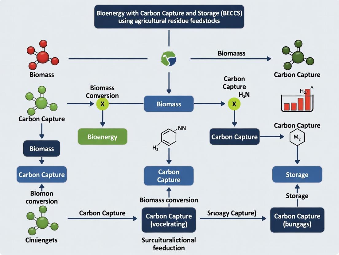
This article examines Bioenergy with Carbon Capture and Storage (BECCS) utilizing agricultural residues as a critical, yet complex, pathway for achieving negative emissions.
Agricultural Residue BECCS: A Viable Path to Negative Emissions and Bioenergy Security
Abstract
This article examines Bioenergy with Carbon Capture and Storage (BECCS) utilizing agricultural residues as a critical, yet complex, pathway for achieving negative emissions. Tailored for researchers and sustainability scientists, it explores the foundational science of residue conversion, details current capture methodologies, addresses technical and supply chain challenges, and validates performance through comparative life-cycle and techno-economic analyses. The synthesis provides a comprehensive roadmap for integrating agricultural waste into climate mitigation strategies, highlighting key research gaps and implementation priorities.
The Science and Promise of Agricultural Waste in Carbon-Negative Systems
This application note provides a standardized framework for characterizing agricultural residue feedstocks within Bioenergy with Carbon Capture and Storage (BECCS) research. Accurate definition of feedstock type, availability, and carbon content is fundamental for modeling carbon negativity, designing conversion processes, and assessing global scalability.
Types and Characterization of Key Residues
Agricultural residues are classified as primary (field residues like stalks) or secondary (processing residues like husks). Key feedstocks for thermochemical BECCS pathways (e.g., gasification, pyrolysis) include:
Cereal Straws: Wheat, rice, maize, and barley straws are predominant. They exhibit high cellulose/hemicellulose content and moderate ash. Stover: Corn and maize stover, consisting of cobs, leaves, and stalks, are bulkier with variable moisture. Husks & Shells: Rice husks, nut shells (e.g., coconut, almond) have higher lignin and ash (especially silica in rice husk). Bagasse: Fibrous matter from sugarcane processing, with high moisture at point of generation. Prunings: From perennial crops (e.g., olive, vine) are seasonal and heterogeneous.
Global Availability and Carbon Content Data
Quantitative data on annual global production (residue-to-product ratio based) and characteristic carbon content are summarized. Values are estimated means; local variability is significant.
Table 1: Global Annual Availability & Carbon Content of Key Residues
| Feedstock Type | Estimated Global Annual Production (Million tonnes, dry basis) | Typical Carbon Content (% dry basis) | Key Producing Regions |
|---|---|---|---|
| Rice Straw | 550 - 750 | 38 - 42 | Asia (China, India, SE Asia) |
| Wheat Straw | 450 - 600 | 40 - 45 | Asia, Europe, North America |
| Maize Stover | 400 - 600 | 42 - 47 | North America, Asia, South America |
| Sugarcane Bagasse | 180 - 250 | 45 - 50 | Brazil, India, China |
| Rice Husk | 120 - 180 | 35 - 40 | Asia (China, India, SE Asia) |
| Barley Straw | 80 - 120 | 40 - 44 | Europe, Russia, Australia |
| Nut Shells (Aggregate) | 15 - 30 | 48 - 55 | Varied (Asia, Americas) |
Note: Availability considers sustainable removal rates (typically 30-70% of total residue to protect soil health). Data synthesized from FAOStat, IEA Bioenergy reports, and recent literature (2022-2024).
Table 2: Proximate & Ultimate Analysis Ranges for BECCS Modeling
| Feedstock | Fixed Carbon (% db) | Volatile Matter (% db) | Ash (% db) | HHV (MJ/kg db) | N (% db) |
|---|---|---|---|---|---|
| Wheat Straw | 15 - 20 | 70 - 75 | 4 - 8 | 16 - 18 | 0.5 - 0.8 |
| Rice Husk | 18 - 23 | 60 - 65 | 15 - 22 | 14 - 16 | 0.3 - 0.6 |
| Maize Stover | 16 - 21 | 71 - 76 | 5 - 9 | 17 - 18.5 | 0.6 - 1.0 |
| Sugarcane Bagasse | 14 - 18 | 74 - 78 | 2 - 6 | 17 - 19 | 0.2 - 0.4 |
Experimental Protocols for Feedstock Characterization
Protocol 4.1: Determination of Sustainable Availability at Regional Scale
Objective: To estimate technically and sustainably harvestable residue for a given crop in a defined region. Materials: Regional crop production data (FAO/National stats), GIS software, soil type maps, residue-to-product ratios (RPR) from literature. Method:
- Acquire annual crop yield data (tonne/ha) for the target region for a 5-year average.
- Apply region-specific RPR (e.g., 1.4 for maize stover, 1.2 for wheat straw) to calculate total residue generated.
- Apply sustainability constraint factors: Determine fraction removable based on soil organic carbon maintenance, erosion prevention, and agronomic use. Use model-based factors (e.g., 0.4 for erosion-prone land, 0.7 for low-risk land).
- Calculate technically recoverable residue by applying machinery recovery efficiency factors (typically 0.6-0.8).
- Output: Map or table of sustainably harvestable dry tonne/year per sub-region.
Protocol 4.2: Standardized Feedstock Sampling & Preparation (ISO/ASTM Based)
Objective: To obtain a representative, homogeneous sample for compositional analysis. Materials: Sample bags (paper, breathable), jaw crusher, rotary mill (with sieve sets), desiccator, moisture analyzer, sample dividers. Method:
- Field Sampling: For field residues, use a randomized quadrant sampling method across the field. Collect minimum 10 sub-samples (≥1 kg each). Combine into a gross sample.
- Air Drying: Dry gross sample in a ventilated oven at ≤40°C until moisture <15% to prevent biodegradation.
- Size Reduction & Homogenization: Coarse crush to <10 mm. Use a coning and quartering or mechanical sample divider to obtain a representative lab sample (~500g). Mill a subset to <0.5 mm for chemical analysis, and <1.0 mm for thermal analysis.
- Storage: Store milled samples in airtight containers in a desiccator or freezer to prevent moisture uptake and degradation.
Protocol 4.3: Determination of Carbon Content via Elemental (Ultimate) Analysis
Objective: To accurately measure the total carbon mass fraction in the feedstock. Materials: Elemental analyzer (CHNS/O), tin/capsule sample cups, certified reference material (e.g., acetanilide), high-purity gases (He, O2), microbalance (0.001 mg accuracy). Method:
- Calibration: Weigh ~2-3 mg of certified reference material into a tin cup. Run 3-5 replicates to establish calibration curve for carbon detection.
- Sample Preparation: Pre-dry milled sample at 105°C for 2 hrs. Cool in desiccator. Precisely weigh 2-3 mg of dried sample into a tin cup. Crimp tightly.
- Combustion & Analysis: Load sample into the auto-sampler. The analyzer combusts the sample at ~1000°C in oxygen, reduces combustion gases, and separates/quantifies CO2 via gas chromatography/thermal conductivity detection.
- Calculation: The instrument software reports carbon content as a percentage of the dry sample mass based on the calibration curve. Report mean of triplicate analyses with standard deviation.
- QA/QC: Include a blank and a check standard every 10 samples. Recovery for the check standard should be within 98-102%.
Visualization of Workflows and Relationships
Feedstock Characterization Workflow for BECCS Research
Feedstock Screening for Thermochemical BECCS Pathways
The Scientist's Toolkit: Key Research Reagents & Materials
Table 3: Essential Reagents and Materials for Feedstock Analysis
| Item Name | Specification / Example | Primary Function in Protocol |
|---|---|---|
| Elemental Analyzer Standards | Acetanilide, BBOT, Aspartic Acid | Calibration and verification of carbon, hydrogen, nitrogen, and sulfur measurements. |
| Ash Crucibles | Porcelain or platinum, high-form | Used in proximate analysis for determination of ash content via muffle furnace combustion. |
| Anhydrous Magnesium Perchlorate [Desiccant] | ACS grade, for desiccators | Maintains a dry environment for cooling and storing moisture-sensitive samples after drying. |
| Inert Sample Cups | Tin or Silver capsules for CHNS | Encapsulation of solid samples for complete and controlled combustion in the elemental analyzer. |
| Certified Reference Biomass | NIST SRM 849x series (e.g., Poplar) | Quality control material to validate the accuracy of proximate, ultimate, and compositional analyses. |
| Silica Gel | Indicating, 2-5 mm mesh | Desiccant for storage of prepared samples to prevent moisture uptake prior to analysis. |
| Sieve Set | ASTM E11 Standard, 0.5mm & 1.0mm apertures | Standardized particle size reduction for homogeneous sub-sampling and representative analysis. |
| Extraction Thimbles | Cellulose, Soxhlet extraction | Used in solvent extraction protocols for determination of extractives content (e.g., ASTM D1105). |
Application Notes: BECCS with Agricultural Residues
Bioenergy with Carbon Capture and Storage (BECCS) is a negative emissions technology central to IPCC climate mitigation pathways. When applied to agricultural residues (e.g., corn stover, wheat straw, rice husks), it leverages recently fixed atmospheric CO₂, which, when combined with carbon capture during energy conversion and subsequent geological storage, results in net carbon removal.
Key Feedstock Characteristics & Availability
The viability of agricultural residue-based BECCS hinges on sustainable harvest rates, logistics, and biochemical composition affecting conversion efficiency.
Table 1: Global Annual Availability and Characteristics of Major Agricultural Residues
| Residue Type | Estimated Global Annual Availability (Mt dry matter) | Sustainable Harvestable Fraction (%) | Average Lower Heating Value (MJ/kg) | Average Carbon Content (% dry basis) |
|---|---|---|---|---|
| Corn Stover | 1280 | 30-50 | 17.5 | 45-48 |
| Wheat Straw | 1050 | 30-40 | 17.2 | 44-47 |
| Rice Husk | 770 | 60-80 | 15.5 | 38-42 |
| Sugarcane Bagasse | 540 | 70-90 | 18.0 | 46-49 |
Sources: IEA Bioenergy (2023), IPCC AR6 (2022), recent global biomass assessments.
Net Carbon Removal Potential
The net removal is calculated as: Captured CO₂ from flue gas minus Supply chain emissions minus Indirect Land-Use Change (iLUC) emissions.
Table 2: Estimated Carbon Removal Potential per Feedstock Type
| Feedstock | System Boundary | Estimated Net CO₂ Removal (tCO₂/t dry feedstock) | Key Uncertainties & Notes |
|---|---|---|---|
| Corn Stover | Farm-to-Storage | 0.6 - 0.9 | Highly sensitive to soil carbon repayment from removal. |
| Wheat Straw | Farm-to-Storage | 0.5 - 0.8 | Dependent on residue management practices. |
| Rice Husk | Farm-to-Storage | 0.8 - 1.1 | Higher ash content challenges conversion efficiency. |
| Sugarcane Bagasse | Farm-to-Storage | 0.9 - 1.2 | Often considered a processing byproduct, lower iLUC risk. |
Note: Ranges reflect variations in supply chain efficiency, capture rate (85-95%), and geological storage integrity.
Experimental Protocols
Protocol: Life Cycle Assessment (LCA) for BECCS System Analysis
Objective: Quantify the net greenhouse gas (GHG) balance of a BECCS value chain using a specific agricultural residue.
Methodology:
- Goal & Scope Definition: Define functional unit (e.g., 1 MWh electricity or 1 t dry feedstock). Set system boundaries (cradle-to-grave: cultivation, harvest, transport, pre-treatment, conversion, CCS, storage).
- Inventory Analysis (LCI):
- Feedstock Production: Collect data on fertilizer inputs, diesel for harvesting, and changes in soil organic carbon (SOC) using models like DAYCENT or IPCC Tier 2 methods.
- Logistics: Model transport distances, modes, and energy use for collection, densification, and delivery.
- Conversion & CCS: Use process simulation software (e.g., Aspen Plus) for a biomass-fired power plant with post-combustion amine-based capture (e.g., 30 wt% MEA). Obtain mass/energy balances. Include capture solvent manufacturing and degradation.
- Storage: Model pipeline transport and injection energy. Assume 99% permanence over 1000 years.
- Impact Assessment: Calculate Global Warming Potential (GWP) using IPCC AR6 factors. Net CO₂ removal = (Biogenic CO₂ captured + stored) - (Total supply chain GHG emissions).
- Interpretation & Sensitivity Analysis: Test sensitivity to key parameters: SOC change, capture rate, grid electricity carbon intensity, and transport distance.
Protocol: Laboratory-Scale Biomass Gasification with Syngas CO₂ Capture
Objective: Determine the CO₂ yield and capture efficiency from the gasification of milled agricultural residue.
Materials: See Scientist's Toolkit. Procedure:
- Feedstock Preparation: Dry feedstock at 105°C for 24h. Mill and sieve to 500-800 µm.
- Gasification: Load 100g feedstock into a fluidized-bed gasifier reactor. Purge with N₂. Heat to 850°C under controlled N₂ flow (1 L/min). Introduce steam (0.5 kg/h) as gasification agent.
- Syngas Conditioning: Pass raw syngas through a series of condensers (0°C) and filters (glass wool, 5 µm) to remove tars and particulate matter.
- CO₂ Capture Unit: Direct cleaned syngas into a packed-bed absorption column (height: 50 cm, diameter: 5 cm) containing 500 mL of 3M Monoethanolamine (MEA) solution at 40°C. Operate in counter-current flow mode.
- Measurement & Analysis:
- Online Gas Analysis: Use inline NDIR CO₂ sensor pre- and post-absorption column to measure CO₂ concentration continuously.
- Capture Efficiency Calculation: Record volumetric flow rates and concentrations. Calculate: Capture Efficiency (%) = [(CO₂in - CO₂out) / CO₂_in] * 100.
- Solvent Regeneration: Heat rich solvent to 120°C in a separate flask to desorb CO₂. Measure desorbed CO₂ volume using a gasometer.
- Data Recording: Record temperature, pressure, flow rates, and CO₂ concentrations at 5-minute intervals for a minimum of 1 hour of stable operation.
Visualizations
BECCS Carbon Flow from Biomass to Storage
LCA Workflow for BECCS Carbon Accounting
The Scientist's Toolkit: Key Research Reagent Solutions
Table 3: Essential Materials for BECCS Laboratory Research
| Item / Reagent | Function & Application | Example Vendor / Specification |
|---|---|---|
| Milled Agricultural Residue | Standardized feedstock for gasification/pyrolysis experiments. Particle size critical for kinetics. | In-house prepared, sieved to 500-800 µm. |
| Monoethanolamine (MEA) Solution | Benchmark solvent for post-combustion CO₂ capture in absorption/desorption experiments. | Sigma-Aldrich, 30 wt% in H₂O, reagent grade. |
| Fluidized Bed Gasifier (Lab-Scale) | Enables controlled thermochemical conversion of biomass under various atmospheres (steam, O₂). | Custom or from specialist manufacturers (e.g., Carbolite Gero). |
| Online NDIR CO₂ Analyzer | Real-time measurement of CO₂ concentration in gas streams pre- and post-capture. | Vaisala CARBOCAP or Siemens Ultramat 23. |
| Aspen Plus Process Simulator | Software for modeling mass/energy balances of full-scale BECCS plant configurations. | AspenTech. |
| Soil Organic Carbon (SOC) Model | Quantifies carbon debt from residue removal (critical for LCA). | DAYCENT model or IPCC Inventory Software. |
Within the strategic framework of Bioenergy with Carbon Capture and Storage (BECCS), the utilization of agricultural residues as feedstocks presents a critical pathway for achieving negative carbon emissions. While corn stover and rice husks are well-characterized, a broader array of underutilized residue streams offers significant potential to enhance biomass availability, diversify supply chains, and improve the sustainability profile of BECCS systems. This application note details the characterization, pre-treatment, and conversion protocols for three such underutilized residues: tomato vine waste, cocoa pod husk, and artichoke threshing residue.
Feedstock Characterization: Quantitative Analysis
Recent analyses (2023-2024) of underutilized residues reveal compositional data critical for predicting conversion efficiency and bioenergy yield in BECCS processes. The data is summarized in the table below.
Table 1: Proximate and Ultimate Analysis of Selected Underutilized Residues
| Feedstock | Lignin (% Dry Basis) | Cellulose (% Dry Basis) | Hemicellulose (% Dry Basis) | Ash Content (% Dry Basis) | Higher Heating Value (MJ/kg) | C/N Ratio |
|---|---|---|---|---|---|---|
| Tomato Vine | 18.2 ± 1.5 | 32.5 ± 2.1 | 16.8 ± 1.3 | 10.5 ± 0.8 | 17.1 ± 0.3 | 28:1 |
| Cocoa Pod Husk | 24.7 ± 2.0 | 28.4 ± 1.8 | 20.3 ± 1.5 | 8.3 ± 0.7 | 16.3 ± 0.4 | 35:1 |
| Artichoke Threshing Residue | 15.1 ± 1.2 | 35.8 ± 2.3 | 22.5 ± 1.6 | 14.2 ± 1.0 | 15.8 ± 0.3 | 25:1 |
| Corn Stover (Reference) | 17-21 | 35-40 | 20-25 | 4-6 | 17.5-18.5 | ~40:1 |
Source: Compiled from recent studies in 'Biomass and Bioenergy' and 'Waste and Biomass Valorization' (2023-2024).
Experimental Protocols
Protocol 3.1: Standardized Feedstock Pre-treatment for Enzymatic Saccharification
Objective: To prepare underutilized residues for optimal sugar release via enzymatic hydrolysis, a key step for subsequent fermentation to bioethanol (with integrated carbon capture).
Materials:
- Dried, milled residue (<2 mm particle size).
- Dilute sulfuric acid (1-3% w/w) or sodium hydroxide solution (2% w/w).
- Autoclave or pressurized heating reactor.
- Vacuum filtration setup.
- pH meter and neutralization chemicals (Ca(OH)₂ or H₂SO₄).
- Deionized water.
Methodology:
- Loading: Charge 10g of dry biomass into a 500 mL reactor vessel.
- Impregnation: Add pre-mixed acid or alkali solution at a 10:1 liquid-to-solid ratio.
- Reaction: Seal reactor and heat to 160°C (for acid) or 120°C (for alkali) for 30 minutes under autogenous pressure.
- Quenching & Recovery: Rapidly cool reactor to 50°C. Filter the slurry through a Büchner funnel.
- Washing & Neutralization: Wash solid fraction thoroughly with deionized water until effluent pH is neutral. Record mass of recovered solid (pretreated biomass).
- Analysis: Analyze solid for compositional change (per Table 1 methods) and store at 4°C for hydrolysis.
Protocol 3.2: High-Throughput Enzymatic Hydrolysis & Sugar Yield Assay
Objective: To quantitatively evaluate the saccharification potential of pretreated residues.
Materials:
- Pretreated biomass (from Protocol 3.1).
- Commercial cellulase/hemicellulase cocktail (e.g., CTec3).
- Sodium citrate buffer (50 mM, pH 4.8).
- 96-well deep-well plates and orbital shaker incubator.
- DNS (3,5-dinitrosalicylic acid) reagent or HPLC for sugar quantification.
Methodology:
- Slurry Preparation: Dispense 100 mg (dry weight equivalent) of pretreated biomass into each well.
- Enzyme Loading: Add sodium citrate buffer to achieve 2% (w/v) solids concentration. Add enzyme cocktail at a loading of 20 mg protein/g glucan.
- Incubation: Seal plates and incubate at 50°C with continuous agitation at 150 rpm for 72 hours.
- Sampling: At 0, 6, 24, 48, and 72 hours, remove 100 µL aliquots, centrifuge, and collect supernatant.
- Quantification: Analyze supernatant glucose and xylose concentration using HPLC (Gold standard) or a calibrated DNS assay. Calculate yield as g sugar per 100g raw dry biomass.
Signaling & Process Pathways
Title: BECCS Pathway for Underutilized Agricultural Residues
The Scientist's Toolkit: Research Reagent Solutions
Table 2: Essential Reagents and Materials for Residue Conversion Research
| Item | Function/Benefit | Example/Notes |
|---|---|---|
| CTec3 / HTec3 Enzyme Cocktails | High-efficiency cellulase/hemicellulase blends for saccharification of pretreated lignocellulose. | Novozymes. Critical for quantifying achievable sugar yields. |
| YPD Broth / Agar | Medium for cultivation of fermentative microorganisms (e.g., S. cerevisiae, engineered strains). | Supports bioethanol production trials from hydrolysates. |
| Dionex CarboPac PA1 Column | HPLC column for precise separation and quantification of monomeric sugars (glucose, xylose, arabinose). | Essential for accurate saccharification yield data. |
| 3,5-Dinitrosalicylic Acid (DNS) Reagent | Colorimetric assay for quantifying reducing sugars in hydrolysates. | Rapid, high-throughput screening tool. |
| Lignin Reference Standard (Kraft Lignin) | Standard for calibrating lignin content analysis (e.g., Klason method). | Necessary for compositional analysis. |
| Anaerobic Chamber Gloves/Bags | Maintains anoxic conditions for sensitive fermentation or microbial consortium studies. | Crucial for simulating industrial bioreactor conditions. |
| Solid Residue Sampling Kit | Includes moisture meters, portable grinders, and sterile containers. | Ensures representative and stable field sampling of residues. |
Geospatial Analysis of Residue Availability and Proximity to Storage Sites
Abstract Within the broader thesis on Bioenergy with Carbon Capture and Storage (BECCS) utilizing agricultural residues, this protocol details a geospatial methodology to quantify feedstock availability and optimize pre-processing storage site locations. It provides a replicable framework for integrating disparate data sources—satellite imagery, agricultural statistics, and logistical parameters—into a decision-support model, crucial for supply chain feasibility studies in BECCS deployment.
Application Note: Geospatial Data Integration for BECCS Feedstock Logistics
Objective: To model the spatial and temporal distribution of agricultural residue biomass and identify optimal storage hub locations to minimize transport costs and feedstock degradation for a BECCS facility.
Core Datasets & Pre-processing Protocol Table 1: Primary Geospatial and Statistical Data Requirements
| Data Layer | Source Example | Key Attributes | Pre-processing Step |
|---|---|---|---|
| Land Use/Land Cover (LULC) | USGS Landsat, ESA Sentinel-2 | Crop type classification, harvest dates | Supervised classification (Random Forest) to map residue-producing crops (e.g., corn, wheat). |
| Agricultural Yield Statistics | USDA NASS, FAO STAT | County/district-level crop production (bu/acre, ton/ha) | Spatial disaggregation (dasymetric mapping) using LULC raster to create high-resolution yield maps. |
| Residue-to-Production Ratio (RPR) | Literature Review (e.g., NREL) | Crop-specific coefficients (e.g., Corn Stover: 1.0 dry ton/acre) | Application of RPR to yield maps to generate theoretical residue availability raster. |
| Road Network | OpenStreetMap, TIGER/Line | Road type, speed limit, tolls | Network topology creation, impedance assignment (travel time/cost per segment). |
| Digital Elevation Model (DEM) | SRTM, ASTER GDEM | Elevation, slope | Calculate terrain difficulty factor for transport cost models. |
| Existing Infrastructure | GIS Databases | Location of potential storage sites (e.g., former granaries), protected lands | Buffer analysis to exclude environmentally sensitive areas. |
Key Experimental Workflow: Network Analysis for Site Suitability Protocol 1: Cost-Weighted Distance and Service Area Analysis
- Data Preparation: Convert the residue availability raster to point features representing biomass concentration centroids. Load the road network and potential storage sites as vector layers.
- Network Impedance Modeling: Using GIS software (e.g., ArcGIS Pro, QGIS), assign a cost per unit length to each road segment based on type (e.g., highway, local road) and slope-derived terrain difficulty. Define average truck speed and operating cost for each class.
- Service Area Calculation: For each candidate storage site, run a Network Analysis to determine all biomass points reachable within a specified maximum transport cost or time (e.g., $10/dry ton, 45 minutes). This defines the site's feedstock procurement basin.
- Biomass Aggregation: Sum the available residue tonnage from all points within each procurement basin. This provides the total serviceable feedstock for each candidate site.
- Multi-Criteria Decision Analysis (MCDA): Rank candidate sites using a weighted suitability model (Table 2).
Table 2: MCDA Criteria for Storage Site Selection
| Criterion | Weight (%) | Measurement | Objective |
|---|---|---|---|
| Total Serviceable Feedstock (tons/yr) | 35 | Sum within procurement basin | Maximize |
| Average Transport Cost ($/ton) | 30 | Cost-weighted distance from all serviceable points | Minimize |
| Site Acreage (hectares) | 20 | Area available for storage and handling | Maximize |
| Proximity to Major Roads (km) | 15 | Euclidean distance to nearest highway | Minimize |
Diagram Title: Geospatial Workflow for Biomass Storage Siting
The Scientist's Toolkit: Key Research Reagent Solutions
Table 3: Essential Software & Data Tools for Geospatial BECCS Analysis
| Item / Solution | Function / Role | Example / Vendor |
|---|---|---|
| GIS Platform | Core software for spatial data manipulation, analysis, and cartography. | ArcGIS Pro, QGIS (Open Source) |
| Remote Sensing Software | Processes satellite imagery for crop classification and change detection. | ENVI, Google Earth Engine |
| Network Analyst Extension | Performs network-based routing, service area, and closest facility analysis. | ArcGIS Network Analyst, QGIS pgRouting |
| Spatial Analyst Extension | Conducts raster calculations (e.g., yield disaggregation, cost surfaces). | ArcGIS Spatial Analyst, QGIS Raster Calculator |
| Python (geopandas, arcpy) | Automates repetitive geospatial workflows and data processing pipelines. | Jupyter Notebook, IDE (VS Code, PyCharm) |
| Agricultural Statistics API | Programmatic access to current and historical crop production data. | USDA Quick Stats API, FAO API |
Experimental Protocol: Field Validation of Residue Estimates
Protocol 2: Ground-Truthing and Model Calibration
- Stratified Random Sampling: Based on the residue availability raster, stratify the study area into high, medium, and low availability zones. Randomly generate at least 30 sample points per stratum.
- Field Measurement: At each sample point (within a homogenous field), establish a 1m x 1m quadrant post-harvest.
- Collect all above-ground residue within the quadrant.
- Oven-dry samples at 70°C until constant weight to determine dry matter content.
- Calculate dry tons per acre/hectare.
- Model Calibration: Statistically compare field-measured residue values with model-predicted values at the sample coordinates using linear regression. Use the regression parameters to calibrate (adjust) the initial RPR coefficients, improving the model's predictive accuracy.
Diagram Title: Field Validation Protocol for Residue Models
Fundamental Thermochemical vs. Biochemical Conversion Pathways for Residues
This application note details the experimental characterization of thermochemical and biochemical conversion pathways for agricultural residues (e.g., corn stover, wheat straw) within a BECCS (Bioenergy with Carbon Capture and Storage) research framework. The objective is to provide a comparative analysis of pathways for generating energy and/or platform chemicals while enabling carbon-negative outcomes through coupled carbon capture. Selection of the optimal pathway is critical for the techno-economic viability and life-cycle assessment of large-scale BECCS deployment.
Table 1: Fundamental Characteristics of Conversion Pathways
| Parameter | Thermochemical Pathway (Gasification/Pyrolysis) | Biochemical Pathway (Anaerobic Digestion/ Fermentation) |
|---|---|---|
| Primary Feedstock Suitability | Lignocellulosic residues; high heterogeneity tolerated. | Residues with high carbohydrate (C5/C6) content; lower lignin preferred. |
| Core Process Drivers | High temperature (300–1200°C), pressure, sometimes catalyst. | Microbial/enzymatic action, mild conditions (20–70°C, ambient pressure). |
| Key Intermediate Products | Syngas (CO, H₂), Bio-oil, Biochar. | Soluble sugars (glucose, xylose), biogas (CH₄, CO₂), organic acids. |
| Typical Final Energy Vectors | Heat, electricity, synthetic fuels (FT diesel, H₂). | Biogas (CH₄), bioethanol, biohydrogen. |
| Process Duration | Seconds to minutes (fast pyrolysis) or hours (slow pyrolysis/gasification). | Days (fermentation) to weeks (anaerobic digestion). |
| Net Carbon Efficiency (Feedstock C to Product C) | 60–85% (Gasification to syngas) | 70–90% (Fermentation to ethanol) |
| Carbon Capture Integration Point | Post-combustion of syngas/biogas, or biochar sequestration. | Pre-combustion from biogas upgrade, or post-fermentation CO₂. |
| Key Challenge for BECCS | Tar formation in syngas; gas cleaning for CCS. | Recalcitrance of lignin; slow hydrolysis rates. |
Table 2: Recent Experimental Yields from Corn Stover (2022-2024 Data)
| Conversion Process | Experimental Condition | Primary Product Yield | CO₂ Stream Purity for Capture |
|---|---|---|---|
| Fast Pyrolysis | 500°C, short vapor residence. | Bio-oil: 60-70 wt.% | Low (dilute in flue gas, post-combustion). |
| Steam Gasification | 750°C, catalyst (Na₂CO₃). | Syngas: 1.5 m³/kg (H₂: 35% vol) | High (pre-combustion, ~30% vol in syngas). |
| Enzymatic Hydrolysis + Fermentation | Pretreatment: Dilute acid. Enzymes: 15 FPU/g. | Bioethanol: 280 L/ton dry matter | High (nearly pure from fermentation off-gas). |
| Anaerobic Digestion | Wet process, 35°C, 30 days. | Biogas: 450 m³/ton VS (CH₄: 55%) | Medium (~45% CO₂ in raw biogas). |
Detailed Experimental Protocols
Protocol 1: Thermochemical – Catalytic Steam Gasification for Enhanced H₂/CO₂ Yield
Objective: To produce a hydrogen-rich syngas with a concentrated CO₂ stream amenable to capture from agricultural residue.
Materials: Milled residue (<2 mm), lab-scale fluidized bed reactor, steam generator, Na₂CO₃ catalyst, gas chromatography (GC-TCD), condensate trap.
Procedure:
- Feedstock Preparation: Dry corn stover to <10% moisture. Impregnate with 10 wt.% Na₂CO₃ solution (catalyst), then re-dry.
- Reactor Setup: Load 200g of catalysed feedstock into reactor. Set temperature to 750°C under N₂ purge (1 L/min).
- Steam Introduction: Initiate steam flow (0.5 g H₂O/min) once temperature stabilizes.
- Gas Sampling & Analysis: After 10 minutes of stable steam flow, connect outlet to condensate trap (to remove tars/water). Collect dry gas sample in a Tedlar bag at 15-minute intervals for 1 hour.
- GC Analysis: Analyze gas samples for H₂, CO, CO₂, CH₄ composition using a calibrated GC-TCD.
- Data Calculation: Calculate syngas yield (m³/kg dry feed) and H₂/CO ratio. The CO₂ concentration in the dry syngas is the pre-combustion capture target.
Protocol 2: Biochemical – High-Solid Enzymatic Hydrolysis & Fermentation with CO₂ Off-Gas Monitoring
Objective: To hydrolyze cellulose/hemicellulose to fermentable sugars and convert them to ethanol while collecting high-purity CO₂.
Materials: Dilute-acid pretreated corn stover, commercial cellulase/hemicellulase cocktail, Saccharomyces cerevisiae strain, bioreactor with off-gas condenser, CO₂ analyzer, HPLC.
Procedure:
- Hydrolysis: Load pretreated stover at 20% solids (w/w) into a bioreactor. Adjust pH to 5.0. Add enzyme cocktail at 15 FPU/g cellulose. Incubate at 50°C with mixing (150 rpm) for 72 hours.
- Fermentation Inoculation: Cool hydrolysate to 32°C. Inoculate with S. cerevisiae at 5 g/L cell density. Seal reactor, connect off-gas line to a cooled condenser and then to a calibrated CO₂ analyzer/mass flow meter.
- Monitoring: Monitor CO₂ evolution rate (g/hour) and total volume for 48-72 hours. Periodically sample broth (1 mL) for HPLC analysis (glucose, xylose, ethanol, inhibitors).
- Product Recovery: At endpoint, centrifuge broth. Distill supernatant to recover ethanol. Calculate ethanol yield (g/g sugar consumed). The logged CO₂ mass is the directly capturable stream.
Visualization of Pathways and Workflows
Diagram Title: BECCS Integration Pathways for Agricultural Residues
Diagram Title: Catalytic Gasification & CO2 Capture Workflow
The Scientist's Toolkit: Key Research Reagent Solutions
Table 3: Essential Materials for Residue Conversion Research
| Item Name / Solution | Function in Experiment | Typical Specification / Example |
|---|---|---|
| Cellulase Enzyme Cocktail | Hydrolyzes cellulose to glucose. Essential for biochemical saccharification. | CTec3 or similar; activity ≥ 150 FPU/mL. |
| Na₂CO₃ / K₂CO₃ Catalyst | Catalyzes tar reforming and water-gas shift reaction in gasification, increasing H₂ yield. | ACS grade, >99% purity. |
| Dilute Sulfuric Acid | Standard reagent for pretreatment to solubilize hemicellulose and alter lignin structure. | 1-3% (w/w) solution in water. |
| S. cerevisiae Ethanol Red | Robust yeast strain for hexose fermentation, tolerant to inhibitors. | Genetically defined, lyophilized. |
| Gas Chromatograph with TCD & FID | For precise quantification of syngas components (TCD) and organic compounds (FID). | Agilent 7890B or equivalent with appropriate columns. |
| Anhydrous Ethanol Standard | HPLC calibration for quantification of fermentation ethanol yield. | ≥99.8%, HPLC grade. |
| Tedlar Gas Sample Bags | Inert collection and storage of gas samples for subsequent GC analysis. | 1L volume, PTFE fitting, certified clean. |
| NH₄VO₃ Catalyst (for SCR) | Research into catalytic cleaning of syngas (NOx reduction) pre-combustion/capture. | 99.95% trace metals basis. |
From Field to Storage: Implementing Residue-Based BECCS Systems
Application Notes: Logistics for Agricultural Residue BECCS
Optimizing the supply chain for agricultural residues (e.g., corn stover, wheat straw) is critical for the economic viability and carbon balance of Bioenergy with Carbon Capture and Storage (BECCS). The system's net carbon removal is highly sensitive to logistics emissions. Key phases are interdependent, requiring integrated modeling.
Phase 1: Harvesting & Collection: This initial phase dictates feedstock quality, quantity, and subsequent cost. A multi-pass system (separate grain and residue harvest) is common but incurs higher fuel and labor costs. Single-pass systems, utilizing combined harvesters with residue collection attachments, reduce field operations but may require more sophisticated machinery. Critical decisions include residue removal rate (typically 30-70%) to maintain soil health.
Phase 2: Densification: Low bulk density of residues (~50-80 kg/m³ loose) makes transportation over long distances inefficient. In-field or near-field densification (e.g., baling, pelletization, pyrolysis to bio-oil) increases density (e.g., pellets: ~600 kg/m³). The choice of densification method trades off energy input, cost, and downstream handling ease. Baling (round or square) is standard but results in intermediate density.
Phase 3: Transportation: Models range from direct trucking of bales to centralized depots or biorefineries, to hub-and-spoke systems where multiple satellite storage/densification sites feed a central hub. Transportation emissions (g CO₂e/tonne-km) are a major component of the supply chain footprint. Optimization software is used to determine the most efficient routing and mode (truck, rail).
Integration with BECCS: The entire logistics chain must be analyzed through a Life Cycle Assessment (LCA) lens. Every MJ of fossil fuel used in harvesting, densification, and transport reduces the net carbon negativity of the BECCS operation. Optimal network design minimizes total system cost and emissions per tonne of CO₂ sequestered.
Table 1: Characteristics of Common Densification Methods for Agricultural Residues
| Densification Method | Bulk Density Range (kg/m³) | Typical Energy Input (MJ/tonne) | Key Advantages | Key Disadvantages |
|---|---|---|---|---|
| Loose Chop | 50 - 80 | 5 - 15 | Lowest upfront cost | Very high transport cost, storage issues |
| Round Bales | 120 - 180 | 80 - 120 | Well-established, field-storable | Moderate density, manual handling |
| Square Bales | 180 - 250 | 100 - 150 | Efficient stacking & transport | Higher baler cost |
| Pelletization | 550 - 700 | 500 - 800 | Highest density, flows easily | High capital & energy cost |
| Fast Pyrolysis (Bio-oil) | ~1000 (oil equivalent) | 1500 - 3000 (for conversion) | Liquid fuel, easier to transport | Very high conversion loss & cost |
Table 2: GHG Emissions for Transportation Modes (2023 Estimates)
| Transportation Mode | Average GHG Emission Factor (g CO₂e/tonne-km) | Typical Capacity (tonnes) | Effective Radius |
|---|---|---|---|
| Class 8 Truck | 62 - 85 | 20 - 25 | < 200 km |
| Rail Transport | 22 - 30 | 2000 - 3000 | > 200 km |
| Barge Transport | 15 - 22 | 5000+ | Along waterways |
Experimental Protocols
Protocol 1: Field Measurement of Sustainable Residue Removal Rate Objective: To determine the maximum residue removal rate that preserves soil organic carbon (SOC) for a specific crop and soil type. Materials: Quadrat frame (1m x 1m), precision scale, drying oven, soil corer, soil test kits for SOC. Procedure:
- Post-harvest, randomly place at least 10 quadrats per test field.
- Manually collect all residue within each quadrat.
- Weigh residue, then dry at 70°C to constant weight for dry mass.
- Calculate total residue yield per hectare.
- Using paired plots, remove 30%, 50%, and 70% of this calculated yield. Leave control plots with no removal.
- Annually, using a soil corer, take 0-30 cm soil samples from each plot.
- Analyze SOC content using dry combustion (e.g., CN analyzer).
- Monitor SOC trends over 3-5 years to establish a sustainable removal threshold.
Protocol 2: Life Cycle Assessment (LCA) of a Logistics Pathway Objective: To calculate the gate-to-gate GHG emissions for supplying 1 dry tonne of residue to a BECCS biorefinery. System Boundaries: From standing residue in field to receipt at biorefinery preprocessing hopper. Procedure:
- Define Scenario: Specify harvest method (single/multi-pass), baler type (round/square), transport distance, and mode.
- Collect Inventory Data: a. Fuel consumption (liters/ha) for harvesting, raking, baling. b. Diesel consumption for in-field equipment (l/tonne). c. Transport distance (km) and truck payload (tonnes). d. Electricity use (kWh/tonne) for any stationary densification.
- Apply Emission Factors: Convert all energy inputs to CO₂e using current databases (e.g., GREET model factors). Use Table 2 for transport.
- Calculate: Sum emissions from all unit operations. Express result as kg CO₂e per dry tonne of delivered feedstock.
- Sensitivity Analysis: Vary key parameters (transport distance, removal rate) to model their impact.
Protocol 3: Bulk Density and Durability Testing of Pellets Objective: To evaluate the quality of densified pellets according to ISO standards. Materials: Pellet sample, drying oven, balance, graduated cylinder, pellet durability tester (PDT), sieves (3.15 mm). Procedure:
- Bulk Density (ISO 17828): a. Oven-dry a pellet sample. b. Pour pellets gently into a 1L graduated cylinder from a set height. c. Level the top without compaction. d. Weigh the cylinder's contents. Calculate mass/volume (kg/m³).
- Mechanical Durability (ISO 17831-1): a. Sieve 500g of pellets to remove fines. b. Place sample in the PDT drum. c. Rotate the drum for 500 revolutions at 50 rpm. d. Sieve the sample again on a 3.15 mm sieve. e. Weigh the retained pellets. Durability = (Mass retained / Initial mass) * 100%.
Visualization Diagrams
Title: Agricultural Residue Harvesting and Collection Workflow
Title: LCA Protocol for Logistics Emissions
The Scientist's Toolkit: Research Reagent Solutions
Table 3: Essential Materials for Logistics and Feedstock Analysis
| Item | Function in Research Context |
|---|---|
| CN Elemental Analyzer | Precisely measures carbon and nitrogen content in soil and biomass samples, crucial for calculating carbon balances and soil health impacts. |
| Bomb Calorimeter | Determines the higher heating value (HHV) of feedstock samples, a key parameter for biorefinery energy yield calculations. |
| Portable Soil Moisture Probe | Allows for rapid, in-field measurement of residue and soil moisture, critical for planning harvest timing and drying requirements. |
| GPS Data Logger & GIS Software | Enables precise mapping of field boundaries, residue yield variability, and optimal route planning for collection and transport. |
| Pellet Durability Tester (PDT) | Quantifies the mechanical strength of densified pellets according to ISO standards, predicting handling and storage losses. |
| Custom LCA Software (e.g., openLCA, GREET) | Models the greenhouse gas emissions and energy inputs of complex, multi-step supply chain scenarios. |
| Unmanned Aerial Vehicle (UAV) with Multispectral Camera | Provides remote sensing data to estimate residue cover, biomass yield, and soil conditions at a field scale. |
Within the framework of Bioenergy with Carbon Capture and Storage (BECCS) utilizing agricultural residues, feedstock pre-processing is a critical determinant of system efficiency and carbon negativity. Agricultural residues (e.g., wheat straw, rice husks, corn stover) are heterogeneous, high-moisture, and low-bulk-density materials, posing significant challenges for transport, handling, gasification/combustion, and subsequent carbon capture. This application note details standardized protocols for drying, torrefaction, and pelletization to transform raw biomass into a homogeneous, energy-dense, and stable feedstock suitable for advanced BECCS value chains, thereby enhancing system reliability and net carbon removal potential.
Table 1: Comparative Analysis of Pre-processing Stages for Agricultural Residues
| Process Stage | Primary Objective | Key Operational Parameters | Typical Output Characteristics (for wheat straw) | Impact on BECCS Value Chain |
|---|---|---|---|---|
| Drying | Reduce moisture to enable further processing & prevent degradation. | Temp: 105-120°C; Time: 1-4 hrs; Moisture Target: <10% (w.b.). | Moisture Content: <10%; Energy Density: ~15 MJ/kg (LHV); Mass Yield: ~92-96%. | Reduces transport mass, prevents biological decay, essential for torrefaction. |
| Torrefaction | Improve grindability, hydrophobicity, and energy density via mild pyrolysis. | Temp: 200-300°C; Atmosphere: N₂ or O₂-lean; Residence Time: 10-60 min. | Solid Mass Yield: 60-80%; Energy Yield: 75-90%; O/C Ratio: Reduced by 20-50%. | Produces stable, coal-like fuel; reduces milling energy; improves gasifier syngas quality. |
| Pelletization | Increase bulk density for efficient transport and handling. | Die Temp: 80-100°C; Pressure: 100-300 MPa; Binder: Optional (e.g., starch, 1-3%). | Bulk Density: 600-750 kg/m³; Durability Index: >95%; Pellet Density: ~1200 kg/m³. | Enables automated feeding in gasifiers; reduces storage volume; minimizes dust. |
Table 2: Feedstock Property Evolution Through Pre-processing
| Property | Raw Straw | After Drying | After Torrefaction (250°C) | After Pelletization (Torr. Pellets) |
|---|---|---|---|---|
| Moisture Content (% w.b.) | 15-25 | <10 | 1-3 | 3-5 |
| Bulk Density (kg/m³) | 60-100 | 70-110 | 150-200 | 600-750 |
| Higher Heating Value (MJ/kg, d.b.) | 17-19 | 18-19 | 21-24 | 21-24 |
| Volatile Matter (% d.b.) | 70-80 | ~75 | 55-70 | 55-70 |
| Fixed Carbon (% d.b.) | 15-20 | ~18 | 25-35 | 25-35 |
Detailed Experimental Protocols
Protocol 3.1: Convective Oven Drying for Feedstock Preparation Objective: To standardize moisture reduction of agricultural residues to a target of <10% wet basis. Materials: Forced-air convection oven, analytical balance (±0.01g), moisture pans, crucible tongs, desiccator, raw biomass. Procedure:
- Record the mass of an empty, clean moisture pan (M_pan).
- Place approximately 50g of representative, chopped biomass (<10mm) into the pan. Record the total mass (M_initial).
- Place the pan in the oven preheated to 105±2°C.
- Dry for a minimum of 4 hours, or until constant mass is achieved (mass change <0.1% over 1 hour).
- Using tongs, transfer the pan to a desiccator to cool to room temperature (~30 min).
- Record the final mass (M_final).
- Calculate Moisture Content (MC, % w.b.) = [(Minitial - Mfinal) / (Minitial - Mpan)] * 100.
Protocol 3.2: Bench-Scale Fixed-Bed Torrefaction Objective: To produce torrefied biomass under controlled inert atmosphere at temperatures between 200-300°C. Materials: Horizontal or vertical tube furnace, quartz reactor tube, N₂ gas cylinder with flowmeter, thermocouples, data logger, sample crucible, gas scrubber (optional). Procedure:
- Load 20-50g of pre-dried (<10% MC) biomass into the sample crucible.
- Place the crucible in the center of the reactor tube. Seal the system.
- Purge the reactor with N₂ at a flow rate of 1 L/min for 15 minutes to establish an inert atmosphere.
- Initiate furnace heating at a ramp rate of 10°C/min to the target torrefaction temperature (e.g., 250°C).
- Maintain the target temperature and N₂ flow (0.5 L/min) for the desired residence time (e.g., 30 min).
- After the holding period, rapidly cool the reactor by sliding it out of the furnace or initiating cooling while maintaining N₂ flow.
- Once cool (<50°C), remove the crucible and weigh the torrefied biomass. Calculate mass yield.
- Collect solid product for subsequent analysis (proximate/ultimate analysis, grindability) or pelletization.
Protocol 3.3: Single-Die Pelletization Unit Operation Objective: To produce dense pellets from raw or torrefied biomass, with or without binders. Materials: Laboratory-scale single-die pellet press (e.g., hydraulic press with heated die), hammer mill with 1mm screen, balance, binder solution (e.g., 5% starch gel), calipers. Procedure:
- Mill the feedstock (dried or torrefied) to a particle size of <1mm.
- (Optional) Homogeneously mix in binder solution to achieve target addition rate (e.g., 2% starch by dry mass). Adjust moisture content of mixture to 8-12%.
- Pre-heat the pellet die to 90±5°C.
- Weigh a precise mass of feedstock (e.g., 1.0g) and load it into the die cavity.
- Apply pressure gradually using the hydraulic press. Hold at the target pressure (e.g., 150 MPa) for a dwell time of 30 seconds.
- Eject the pellet and allow it to cool in ambient air.
- Measure pellet dimensions and mass to calculate density. Perform mechanical durability tests per ASABE S269.5.
Visualizations
Diagram 1: BECCS Feedstock Pre-processing Workflow
Diagram 2: Property Evolution Pathways
The Scientist's Toolkit: Research Reagent Solutions & Essential Materials
Table 3: Essential Materials for Feedstock Pre-processing Research
| Item | Function in Research | Typical Specification/Example |
|---|---|---|
| Forced Convection Oven | Precise and uniform drying of biomass samples. | Temperature range: 30-300°C, ±1°C stability. |
| Tube Furnace with Reactor | Controlled thermal treatment (torrefaction) under inert atmosphere. | Max Temp: 1200°C, with programmable controller; Quartz reactor tube. |
| Inert Gas Supply (N₂) | Creates oxygen-free environment for torrefaction, preventing combustion. | High-purity (>99.99%) nitrogen with pressure regulator and flow meter. |
| Laboratory Pellet Press | Forms biomass powder into densified pellets for property testing. | Hydraulic, with heated dies and pressure gauge (capability >200 MPa). |
| Analytical Balance | Accurate measurement of mass yields for all processes. | Capacity 500g, readability 0.01mg. |
| Hammer Mill / Grinder | Reduces particle size for homogenous feedstock and pelletization. | Variable speed, with interchangeable sieves (0.5-2.0mm). |
| Proximate Analyzer (TGA) | Measures moisture, volatile matter, fixed carbon, and ash content. | Thermogravimetric analyzer with controlled atmosphere. |
| Bomb Calorimeter | Determines the higher heating value (HHV) of raw and processed feedstocks. | Isoperibolic or adiabatic, with benzoic acid calibration. |
| Pellet Durability Tester | Quantifies mechanical strength of pellets post-production. | Standardized tumbler box per ASABE/EN norms. |
Application Notes: Integration with Biomass Conversion for BECCS
The integration of carbon capture (CC) technologies with biomass conversion processes is the core engineering challenge for achieving negative emissions via Bioenergy with Carbon Capture and Storage (BECCS). Utilizing agricultural residues (e.g., straw, husks, stover) as feedstocks introduces specific constraints, including high alkali and ash content, variable composition, and lower energy density. The selection and tailoring of CC technology are paramount for system efficiency and economic viability.
Post-Combustion Capture (PCC) is the most readily applicable to existing or new-build biomass power plants. It separates CO₂ from the flue gas after combustion, typically using amine-based solvents. For biomass flue gases, key considerations are the presence of trace contaminants (SOx, NOx, particulates) which degrade solvents, requiring robust pre-cleaning. The lower partial pressure of CO₂ in biomass flue gas (compared to coal) can reduce absorption efficiency.
Oxy-fuel Combustion involves burning biomass in an atmosphere of nearly pure oxygen, diluted with recycled flue gas, resulting in a flue gas stream highly concentrated in CO₂ and water vapor. This method is highly effective for biomass but demands a dedicated, energy-intensive Air Separation Unit (ASU) and careful control of combustion temperature. The high alkali content in agricultural residue ash can exacerbate slagging and fouling under oxy-fuel conditions.
Pre-Combustion Capture involves gasifying the biomass feedstock to produce a syngas (a mixture of H₂, CO, and CO₂). The CO is then shifted with steam to produce more H₂ and CO₂. The CO₂ is separated, leaving a hydrogen-rich fuel for combustion or use in fuel cells. This pathway is complex but offers potential for high-efficiency power generation or biohydrogen production. The challenge lies in tar management and adapting gas cleanup systems for biomass-derived syngas.
Table 1: Comparative Analysis of CC Technologies for Agricultural Residue Conversion
| Parameter | Post-Combustion (Amine-based) | Oxy-fuel Combustion | Pre-Combustion (IGCC pathway) |
|---|---|---|---|
| Technology Readiness Level (TRL) | 9 (Commercial) | 7-8 (Demonstration) | 6-7 (Pilot for biomass) |
| Typical CO₂ Capture Rate (%) | 85-90 | >90 | 85-95 |
| CO₂ Purity in Output Stream (%) | >99.5 | >95 (after drying) | >95-99 |
| Key Energy Penalty Source | Solvent regeneration (2.1-2.5 GJ/t CO₂) | Air Separation (0.7-1.1 GJ/t O₂) & compression | Gasification, ASU, & shift reactor |
| *Estimated Efficiency Penalty (%-points) | 8-12 | 7-10 | 6-9 |
| Major Challenge (Biomass-specific) | Solvent degradation from impurities | Combustion stability & ash behavior | Tar cracking & syngas cleanup |
| Capital Cost Relative Index | 1.0 (Baseline) | 1.3 - 1.5 | 1.5 - 2.0 |
| Best Suited For | Retrofitting existing plants | New-build, high-purity CO₂ streams | Polygeneration (H₂, power, fuels) |
*Based on net electrical efficiency reduction for a biomass power plant.
Experimental Protocols for BECCS Pathway Evaluation
Protocol 2.1: Bench-Scale Post-Combustion Capture with Simulated Biomass Flue Gas
Objective: To evaluate the absorption efficiency and solvent stability of a novel amine blend (e.g., CESAR-1: AMP/PZ) when exposed to a synthetic flue gas containing trace contaminants representative of wheat straw combustion.
Materials & Equipment:
- Gas blending system (mass flow controllers)
- Absorber column (packed bed, 1 m height)
- Desorber/regenerator column (with reboiler)
- Condenser unit
- Online GC or NDIR CO₂ analyzer
- Aqueous amine solvent (2M AMP/1M PZ)
- Gas cylinders: N₂, CO₂, O₂, SO₂ (1000 ppm in N₂), NO (1000 ppm in N₂)
- Peristaltic pumps, thermocouples, pH meter
Methodology:
- Flue Gas Simulation: Prepare a synthetic flue gas mixture of 12% CO₂, 6% O₂, 500 ppm SO₂, 200 ppm NO, balance N₂. Maintain total flow at 1 L/min.
- Absorption Cycle: Pre-heat the flue gas to 40°C. Circulate the solvent (20°C) from the reservoir to the top of the absorber at 50 mL/min, counter-current to the rising gas.
- Monitoring: Measure CO₂ concentration at absorber inlet and outlet continuously. Capture efficiency is calculated as
[(CO2_in - CO2_out)/CO2_in] * 100. - Rich Solvent Loading: After steady-state is reached (≈30 min), sample the "rich" solvent exiting the absorber. Determine CO₂ loading via barium chloride precipitation titration.
- Regeneration: Pump the rich solvent to the desorber column. Apply heat via the reboiler to maintain solvent temperature at 110-120°C for 60 minutes. Capture and measure the evolved CO₂.
- Degradation Study: Repeat cycles 1-5 for 72 hours of continuous operation. Take periodic solvent samples for analysis via Total Inorganic Carbon (TIC) and Ionic Chromatography (IC) to quantify nitrosamine/amine degradation products and heat-stable salt formation.
Protocol 2.2: Oxy-fuel Combustion of Rice Husk in a Drop-Tube Furnace
Objective: To characterize combustion performance and ash deposition propensity of milled rice husk under O₂/CO₂ atmospheres compared to conventional O₂/N₂.
Materials & Equipment:
- Drop-tube furnace (DTF) with controllable temperature zones (up to 1400°C)
- O₂, CO₂, N₂ gas supplies and blending system
- Biomass feeder (vibratory or screw type)
- Ash collection probes (deposition and ultimate collection)
- Scanning Electron Microscope with Energy Dispersive X-ray Spectroscopy (SEM-EDX)
- X-ray Diffraction (XRD) analyzer
- Rice husk feedstock, milled to 150-200 μm.
Methodology:
- Atmosphere Setup: Establish two test atmospheres: i) Conventional: 21% O₂ / 79% N₂. ii) Oxy-fuel: 30% O₂ / 70% CO₂ (to simulate recycled flue gas).
- Combustion Run: Set furnace wall temperature to 1000°C. Introduce feedstock at a constant rate of 0.5 g/min. Allow system to stabilize for 15 minutes.
- Ash Sampling: Insert a water-cooled deposition probe (surface temp ~600°C) into the gas stream for 60 minutes. Collect remaining fly ash in a downstream filter.
- Analysis:
- Burnout: Calculate from mass balance of char collected.
- Ash Deposition: Weigh the deposit on the probe. Analyze deposit morphology and composition via SEM-EDX.
- Ash Fusibility: Analyze filter-collected ash chemistry and determine initial deformation temperature under reducing atmosphere.
- Mineral Transformation: Use XRD on powdered ash to identify crystalline phases (e.g., cristobalite, potassium silicates).
Protocol 2.3: Pre-Combustion Sorption-Enhanced Water-Gas Shift (SEWGS)
Objective: To test a bifunctional catalyst-sorbent material for in-situ CO₂ removal during the water-gas shift reaction of biomass-derived syngas, concentrating the H₂ product stream.
Materials & Equipment:
- High-pressure fixed-bed reactor system (Hastelloy, 1/2" diameter)
- Back-pressure regulator, downstream gas sampling loop
- Online micro-GC for H₂, CO, CO₂, CH₄ analysis
- Syngas mixture cylinder (40% H₂, 30% CO, 20% CO₂, 10% CH₄)
- SEWGS material (e.g., K-promoted hydrotalcite with Pt/WGS catalyst)
- High-precision syringe pump for steam injection
Methodology:
- Reactor Loading: Pack 5g of SEWGS pellets into the isothermal zone of the reactor. Load quartz wool on both ends.
- Pre-treatment: Under N₂ flow (100 mL/min), heat to 300°C for 1 hour to remove physisorbed water.
- Reaction Cycle:
- Adsorption/Shift Phase: Switch feed to simulated wet syngas. Introduce steam via syringe pump at a H₂O:CO molar ratio of 3:1. Maintain total pressure at 20 bar, temperature at 400°C. Monitor outlet gas composition every 2 minutes. The CO₂ will be adsorbed, driving the WGS reaction (CO + H₂O → CO₂ + H₂) towards high-purity H₂ production (>95% dry basis).
- Breakthrough Detection: When CO₂ concentration at the outlet exceeds 1% (breakthrough), stop the syngas feed.
- Regeneration: Switch to a 100% N₂ purge at 400°C to desorb weakly held CO₂. Then perform a pressure swing or temperature swing regeneration (e.g., reduce pressure to 1 bar or increase temperature to 500°C) to fully regenerate the sorbent. Capture the desorbed CO₂ stream.
- Cyclic Stability: Repeat steps 3-4 for 50 cycles. Monitor and record the CO conversion and H₂ purity at the start of each adsorption phase to assess sorbent/catalyst stability.
Diagrams
BECCS Technology Pathways from Biomass to Storage
Post-Combustion Capture Process Workflow
The Scientist's Toolkit: Key Research Reagent Solutions & Materials
Table 2: Essential Materials for BECCS-CC Experimental Research
| Item Name | Function & Relevance | Example Product / Specification |
|---|---|---|
| Amino Solvents (Blends) | Reactive absorbents for post-combustion CO₂ capture. Tailored blends (e.g., AMP/PZ) offer improved kinetics, capacity, and degradation resistance. | CESAR-1 (30% AMP/10% PZ), 5M MEA (benchmark), KS-1 (hindered amine). |
| High-Temperature Sorbents | Solid materials for pre-combustion or direct air capture, often operating on pressure/temperature swing principles. | K-promoted Hydrotalcite, CaO-based sorbents, Zeolite 13X, Metal-Organic Frameworks (MOFs). |
| Biomass Reference Materials | Standardized, characterized biomass feeds for reproducible gasification/combustion experiments. | NIST Willow Shrub (SRM 8496), University of Vienna Beech Wood Char. |
| Synthetic Flue Gas Mixtures | Calibrated gas cylinders for simulating precise combustion atmospheres without operating a burner. | 12% CO₂, 6% O₂, 500 ppm SO₂, balance N₂. Custom blends available. |
| Trace Gas Analyzers | Critical for monitoring low concentrations of CO₂, SO₂, NOx, and O₂ in inlet/outlet streams to calculate capture efficiency. | NDIR CO₂ Analyzer (e.g., Vaisala GMP252), FTIR Multi-Gas Analyzer (e.g., Gasmet DX4000). |
| WGS Catalyst-Sorbent Composite | Bifunctional material for Sorption-Enhanced Water-Gas Shift (SEWGS) experiments in pre-combustion setups. | Pt/CeO₂-Al₂O³ catalyst mixed with or coated on hydrotalcite sorbent. |
| Ash Fusion Analyzer | Determines ash melting behavior under controlled atmospheres, critical for oxy-fuel and boiler design. | LECO AF700, capable of reducing and oxidizing atmospheres. |
| Ionic Chromatography (IC) Standards | For quantifying anion (formate, acetate, nitrate, sulfate) and cation (alkali metals) concentrations in solvent or ash leachates. | EPA Method 300.1 Anion Standard Mix, multi-element cation standard. |
Application Notes: Comparative Analysis of BECCS Integration Pathways
This note compares two primary pathways for integrating Bioenergy with Carbon Capture and Storage (BECCS) using agricultural residues. The analysis is framed within a thesis investigating the technical feasibility and carbon accounting of region-specific residue feedstocks.
Table 1: Key Comparative Metrics for BECCS Integration Pathways
| Metric | Co-firing in Existing Coal Power Plants | Dedicated BECCS Facility |
|---|---|---|
| Primary Feedstock | Blended fuel (e.g., 5-20% biomass with coal). | 100% pre-processed agricultural residue (e.g., wheat straw, rice husk). |
| Capital Expenditure (CAPEX) | Lower retrofit costs for boiler/CCS unit. Higher costs for feedstock prep & storage. | Higher greenfield costs. Optimized, integrated design reduces per-unit cost at scale. |
| Technology Readiness Level (TRL) | High (9) for co-firing; Medium-High (7-8) for CCS retrofit on coal flue gas. | Medium (6-7) for fully integrated, biomass-optimized gasification-CCS systems. |
| Net Carbon Removal Potential (tCO₂/MWh) | 0.05 - 0.15 (Highly dependent on co-firing ratio and biomass supply chain emissions). | 0.30 - 0.45 (Optimized for high-efficiency carbon-negative operation). |
| Key Technical Challenge | Inconsistent flue gas composition; Alkali & chlorine-induced slagging/fouling; Fuel feed system adaptation. | Feedstock variability & preprocessing; Tar cracking in gasification; System scale-up. |
| Operational Flexibility | High. Can adjust biomass ratio based on price/availability; base-load capable. | Lower. Economies of scale require steady, high-volume feedstock supply. |
Table 2: Feedstock Preprocessing Requirements (For ~50 MWe equivalent)
| Process Step | Co-firing Protocol | Dedicated BECCS Protocol |
|---|---|---|
| Drying | To ~15-25% moisture content (air or low-temp dryer). | To ~10-15% moisture (efficient dryer integral to feed system). |
| Size Reduction | Coarse chipping (~50 mm). May require pulverization for high % blends. | Fine grinding (<2 mm) for fluidized beds/gasifiers. |
| Leaching/Washing | Often omitted, increasing fouling/corrosion risks. | Recommended for high-K, Cl residues; reduces slagging and ash sintering. |
| Pelletization/Torrefaction | Beneficial for long-distance transport and handling. | Critical for uniform feeding in pressurized gasification systems. |
Experimental Protocols
Protocol A: Simulated Flue Gas Corrosion Testing for Co-firing Environments Objective: To assess high-temperature corrosion rates of boiler superheater materials under co-firing flue gas conditions.
- Reagent Setup: Prepare synthetic flue gas mixture: N₂ (base), 12% CO₂, 3% O₂, 500 ppm SO₂, 200 ppm HCl. Introduce alkali salt aerosols (K₂SO₄, KCl) via a nebulizer into a pre-heated gas stream.
- Sample Preparation: Cut candidate alloy coupons (e.g., 304H, Sanicro 28) to 15x10x2 mm. Polish to a 1 µm finish, clean ultrasonically in acetone/ethanol, and dry.
- Exposure Experiment: Place coupons in a horizontal tube furnace. Expose to simulated flue gas at 600°C ± 5°C for 500 hours. Control gas flow rate at 100 ml/min.
- Post-Exposure Analysis: Cool in N₂ atmosphere. Weigh to determine mass change. Analyze corrosion products using Scanning Electron Microscopy with Energy Dispersive X-ray Spectroscopy (SEM-EDS) and X-ray Diffraction (XRD).
- Data Normalization: Report corrosion rate as µm/year based on metal loss calculated from mass gain and oxide density.
Protocol B: Bench-Scale Fluidized Bed Gasification of Pelletized Residue Objective: To determine syngas composition and tar yield from gasification of pretreated agricultural residue pellets.
- Reactor Setup: Use a continuous feed, electrically heated bubbling fluidized bed reactor (ID: 50 mm, H: 1000 mm). Bed material: 500g olivine sand (300-500 µm).
- Feedstock Preparation: Mill and pelletize wheat straw to 3mm pellets. Dry at 105°C for 24h to <10% moisture. Characterize proximate/ultimate analysis.
- Gasification Run: Fluidize bed with N₂ and heat to 850°C. Introduce steam as gasifying agent (Steam/Biomass ratio = 0.8 w/w). Initiate biomass feed at 1 kg/h. Maintain steady state for 60 mins.
- Gas & Tar Sampling: After steady state, pass product gas through a series of condensers (ice/acetone) and tar-absorbing solvent traps (dichloromethane). Measure permanent gas composition (H₂, CO, CO₂, CH₄, C₂) via online micro-GC every 10 mins.
- Tar Analysis: Recover and quantify tars gravimetrically from solvent. Analyze tar composition via Gas Chromatography-Mass Spectrometry (GC-MS).
Visualization Diagrams
Diagram 1: BECCS Integration Pathway Comparison
Diagram 2: Corrosion Test Experimental Workflow
The Scientist's Toolkit: Key Research Reagent Solutions
Table 3: Essential Materials for BECCS Feedstock & Process Research
| Reagent/Material | Function & Application | Key Specification |
|---|---|---|
| Olivine Sand | Catalytic bed material for fluidized bed gasification experiments. Reduces tar yield. | (Mg, Fe)₂SiO₄; particle size 300-600 µm. |
| Monoethanolamine (MEA) Solution | Benchmark solvent for post-combustion CO₂ capture simulation studies. | 30 wt.% in H₂O for absorption/desorption tests. |
| Synthetic Flue Gas Mixture | Corrosive environment simulation for material testing in co-firing scenarios. | Custom blend: N₂/CO₂/O₂/SO₂/HCl. Certified ±2%. |
| Dichloromethane (DCM) | Solvent for absorbing and recovering tars from gasification product streams. | HPLC grade, for tar quantification and GC-MS analysis. |
| Alkali Salts (KCl, K₂SO₄) | Key components of biomass ash. Used to study fouling/slagging and aerosol generation. | ACS reagent grade, ≥99.0% purity. |
| Certified Gas Mixtures (H₂, CO, CO₂, CH₄ in N₂) | Calibration standards for syngas analysis via Gas Chromatography (GC). | Certified to ±1% of stated value for each component. |
| Torrefied Biomass Reference Material | Standardized feedstock for comparing gasifier performance across studies. | Defined proximate/ultimate analysis and grindability index. |
Within the research framework of Bioenergy with Carbon Capture and Storage (BECCS) utilizing agricultural residues, the management of solid by-products—primarily biochar and ash—is critical for system sustainability, economic viability, and carbon sequestration verification. These materials represent both a potential carbon sink and a source of valuable soil amendments or industrial materials. This document provides application notes and standardized protocols for the characterization, analysis, and application of these by-products, tailored for researchers and scientists in BECCS and related fields.
Proximate and Ultimate Analysis Protocol
Objective: To determine the basic chemical composition and property profile of biochar and ash samples.
Materials:
- Analytical balance (±0.0001 g)
- Muffle furnace
- Elemental (CHNS/O) analyzer
- Desiccator
- Crucibles (porcelain or platinum)
Procedure:
- Moisture Content: Weigh 1g of sample (Wwet) in a pre-weighed crucible. Dry at 105°C for 24 hours. Cool in a desiccator and re-weigh (Wdry). Moisture (%) = [(Wwet - Wdry)/Wwet] x 100.
- Volatile Matter: Place the dried sample from Step 1 in a muffle furnace at 950°C for 6 minutes in a covered crucible. Cool and weigh. Calculate mass loss.
- Ash Content: Heat the residue from Step 2 at 750°C for 6 hours in an open crucible. The remaining mass is the ash.
- Fixed Carbon: Calculate by difference: Fixed Carbon (%) = 100% - (Moisture% + Volatile% + Ash%).
- Ultimate Analysis: Submit dried, homogenized sample to an elemental analyzer for Carbon, Hydrogen, Nitrogen, Sulfur, and Oxygen (by difference) content.
Table 1: Representative Data from Agricultural Residue-Derived By-products
| Parameter | Unit | Corn Stover Biochar (500°C) | Rice Husk Ash (700°C) | Wheat Straw Biochar (550°C) |
|---|---|---|---|---|
| pH | - | 9.2 ± 0.3 | 10.5 ± 0.4 | 8.9 ± 0.2 |
| Specific Surface Area | m²/g | 120 ± 15 | 35 ± 8 | 95 ± 12 |
| Carbon Content | % d.b. | 72.5 ± 2.1 | 12.3 ± 1.5 | 68.4 ± 2.3 |
| H:Corg ratio | mol/mol | 0.35 ± 0.05 | N/A | 0.41 ± 0.06 |
| O:Corg ratio | mol/mol | 0.15 ± 0.03 | N/A | 0.18 ± 0.04 |
| Total Porosity | % | ~60 | ~45 | ~58 |
| Cation Exchange Capacity | cmolc/kg | 35.2 ± 4.1 | 12.1 ± 2.2 | 30.5 ± 3.8 |
| Plant-Available K | g/kg | 8.5 ± 1.0 | 25.3 ± 2.5 | 7.2 ± 0.9 |
d.b. = dry basis; Data compiled from recent literature (2023-2024).
Stability Assessment via Incubation Protocol
Objective: To quantify the biochar carbon stability (persistence) in a simulated soil environment.
Materials:
- Incubation jars with gas-tight septa
- 1M NaOH traps
- Thermostated incubator
- Fine-textured, C-deficient soil (control)
- Gas Chromatograph or Titration setup
Procedure:
- Mix biochar with pre-dried soil at a rate of 2% (w/w). A soil-only control is mandatory.
- Adjust soil-biochar mixture to 60% Water Holding Capacity.
- Place mixture in incubation jar. Include a vial with 10 mL of 1M NaOH to trap mineralized CO2.
- Incubate at 25°C in the dark. Replace NaOH traps at intervals (e.g., 1, 3, 7, 14, 30, 60 days).
- Quantify trapped CO2 via titration with 1M BaCl2 and HCl, or by weighing precipitated BaCO3.
- Calculate cumulative C mineralization and model the stable C fraction.
Application Notes
Soil Amendment for Enhanced Carbon Sequestration
Biochar application to agricultural soil is a core strategy for securing the "C" in BECCS. Key protocols include:
- Application Rate: Based on C sequestration targets and agronomic limits. Typical field trial rates range from 5-20 tonnes/ha.
- Mixing Protocol: For field studies, use a rotary tiller or disc harrow to incorporate biochar uniformly into the top 15-20 cm of soil.
- Co-amendment with Ash: Wood ash can be applied at 1-5 tonnes/ha to adjust soil pH and supply K, P, and Ca. Critical: Avoid ash application to alkaline soils. Conduct a preliminary soil pH test.
Table 2: Contaminant Screening Limits for Safe Land Application
| Element | Maximum Concentration in Biochar/Ash (mg/kg, dry basis) | Common Analytical Method |
|---|---|---|
| Arsenic (As) | 13-100 | ICP-MS |
| Cadmium (Cd) | 1.4-39 | ICP-MS |
| Chromium (Cr) | 93-1200 | ICP-OES |
| Copper (Cu) | 600-4000 | ICP-OES |
| Lead (Pb) | 150-300 | ICP-MS |
| Zinc (Zn) | 700-7400 | ICP-OES |
| PAHs (16 EPA) | 6-20 | HPLC/GC-MS |
Ranges reflect international guidelines (EBC, IBI, national standards). Mandatory analysis prior to field trials.
Material Science Applications
Protocol for Biochar-Based Catalyst Support:
- Activation: Load 10g of crushed biochar (500-800 µm) into a quartz reactor. Under N2 flow, heat to 800°C at 10°C/min. Introduce steam (20% v/v in N2) for 45 minutes to develop porosity. Cool under N2.
- Metal Impregnation: Use incipient wetness impregnation with a metal salt solution (e.g., K2CO3 for K, Fe(NO3)3 for Fe). Dry at 105°C and calcine at 400°C.
Visualizations
Diagram Title: BECCS By-product Management and Utilization Pathways
Diagram Title: Proximate and Ultimate Analysis Workflow
The Scientist's Toolkit: Research Reagent Solutions
Table 3: Essential Materials and Reagents for By-product Research
| Item | Function/Application | Key Considerations |
|---|---|---|
| Elemental Analyzer (CHNS/O) | Quantifies fundamental organic/inorganic composition. | Required for C sequestration calculations and H/C, O/C ratios (stability indices). |
| Brunauer-Emmett-Teller (BET) Analyzer | Measures specific surface area and pore size distribution of biochar. | Critical for evaluating reactivity and catalyst support potential. |
| Inductively Coupled Plasma Spectrometer (ICP-OES/MS) | Detects and quantifies major, minor, and trace metal contaminants. | Mandatory for safety screening prior to land application (see Table 2). |
| 1M Sodium Hydroxide (NaOH) Traps | Absorbs CO2 during mineralization incubation studies. | Used with titration (BaCl2/HCl) to quantify C mineralization. |
| pH/EC Meter with Soil Probe | Measures pH and electrical conductivity of biochar/ash-soil mixtures. | Guides safe application rates; ash is highly alkaline. |
| Polycyclic Aromatic Hydrocarbon (PAH) Standards | Calibration for HPLC/GC-MS analysis of organic contaminants. | Required to assess pyrolysis process quality and product safety. |
| Isotope-Labeled (¹³C) Compounds | Tracers for detailed studies on biochar degradation pathways and interactions. | Enables precise tracking of biochar-C in complex environmental systems. |
Overcoming Technical and Economic Hurdles in Residue-Fed BECCS
The viability of Bioenergy with Carbon Capture and Storage (BECCS) using agricultural residues (e.g., wheat straw, rice husk, corn stover) is critically undermined by severe ash-related challenges during combustion. These feedstocks contain high concentrations of alkali metals (K, Na) and chlorine, which transform into low-melting-point compounds (e.g., alkali silicates, chlorides, sulfates). This leads to accelerated ash fouling (deposits on heat exchanger surfaces) and slagging (molten or fused deposits in the furnace), reducing heat transfer efficiency, increasing corrosion rates, and causing unscheduled plant shutdowns. For BECCS, these operational issues decrease the net energy output and increase the cost of captured CO₂. This application note details protocols for characterizing fuels, simulating ash behavior, and testing mitigation strategies essential for developing robust BECCS systems.
Table 1: Typical Alkali and Chlorine Content in Selected Agricultural Residues
| Feedstock | Potassium (K₂O) [wt.% dry] | Sodium (Na₂O) [wt.% dry] | Chlorine (Cl) [wt.% dry] | SiO₂ [wt.% ash] | Initial Deformation Temp. (Reducing) [°C] |
|---|---|---|---|---|---|
| Wheat Straw | 10 - 20 | 0.2 - 1.5 | 0.3 - 1.5 | 25 - 50 | ~950 - 1050 |
| Rice Husk | 1 - 5 | 0.1 - 0.5 | 0.1 - 0.5 | 85 - 95 | >1300 |
| Corn Stover | 10 - 25 | 0.5 - 2.0 | 0.5 - 1.8 | 30 - 60 | ~900 - 1000 |
| Barley Straw | 5 - 15 | 0.5 - 2.0 | 0.5 - 1.2 | 25 - 45 | ~950 - 1100 |
Table 2: Key Ash Transformation Reactions and Their Impact
| Reaction | Typical Temperature Range | Resulting Compound/Phase | Primary Impact |
|---|---|---|---|
| KCl(g) + SO₂ + ½O₂ + H₂O → K₂SO₄ + HCl | 700 - 900°C | K₂SO₄ (s) | Fouling, Corrosion |
| 2KCl(g) + SiO₂ + H₂O → K₂SiO₃ + 2HCl | >700°C | K-silicates (s, l) | Slagging, Bed Agglomeration |
| K⁺ + Al-Si minerals → K-Al-silicates (e.g., KAlSi₃O₈) | >1000°C | Alkali Alumino-silicates (s) | Can increase ash melting point |
| CaO + SiO₂ + K₂CO₃ → Ca-K-silicates (low m.p.) | 800 - 1100°C | Low-melting eutectics (l) | Severe slagging |
Experimental Protocols
Protocol 1: Fuel Analysis and Ash Preparation Objective: To determine the elemental composition and prepare standardized ash samples for subsequent analysis. Methodology:
- Fuel Milling: Mill the air-dried feedstock to a particle size of <250 µm using a vibratory disc mill.
- Ultimate & Proximate Analysis: Perform using standard ASTM methods (D3172, D3176, D4239). Specifically analyze for Cl via bomb combustion/ion chromatography (ASTM D4208).
- Ash Preparation (Low-Temperature): Ash the fuel in a muffle furnace at 575±25°C (ASTM D3174) for 24 hours to preserve alkali volatiles. Store in a desiccator.
- ICP-OES/MS Analysis: Digest 0.1g of low-T ash in a microwave-assisted acid digestion system (HNO₃/HF/H₂O₂). Analyze the solution via Inductively Coupled Plasma Optical Emission Spectrometry/Mass Spectrometry (ICP-OES/MS) for K, Na, Ca, Mg, P, Si, Al, Fe, S.
Protocol 2: Ash Fusion Behavior and Melting Temperature Determination Objective: To characterize the sintering and melting behavior of ash under simulated combustion atmospheres. Methodology:
- Sample Preparation: Press the low-T ash into a conical cylinder using a standard ash fusion test mold.
- Ash Fusion Test (ASTM D1857): Place the cone in a controlled atmosphere furnace (reducing: 60% CO, 40% CO₂; oxidizing: ambient air). Equip with a digital camera for profile monitoring.
- Temperature Program: Heat at 8±3°C/min from 538°C to a maximum of 1600°C.
- Data Collection: Record the four characteristic temperatures: Initial Deformation (IDT), Softening (ST), Hemispherical (HT), and Fluid (FT). IDT is the most critical for slagging propensity.
Protocol 3: Lab-Scale Deposit Formation and Fouling Propensity Test Objective: To simulate and quantify the initial stages of ash deposition on a heat exchanger surface. Methodology:
- Reactor Setup: Use an electrically heated tube furnace with an alumina reactor tube.
- Probe Configuration: Insert a temperature-controlled air-cooled alloy probe (material: e.g., Sanicro 28) into the hot zone. Maintain probe surface temperature at 450-550°C (typical superheater temp).
- Combustion Simulation: Introduce a synthetic flue gas (N₂, CO₂, O₂, H₂O, SO₂). Continuously feed milled feedstock (<1 mm) at a controlled rate using a screw feeder into the hot gas stream upstream of the probe.
- Experiment Duration: Run for 4-8 hours.
- Post-Test Analysis: a) Deposit Weight: Measure deposit mass per unit area. b) Morphology/Composition: Analyze deposit cross-section via Scanning Electron Microscopy with Energy Dispersive X-ray Spectroscopy (SEM-EDX). c) Adhesion Strength: Perform a controlled shear force test using a calibrated rig.
Diagrams
Ash Formation and Fouling Pathway
Ash Characterization Experimental Workflow
The Scientist's Toolkit: Research Reagent Solutions
Table 3: Essential Materials and Reagents for Combustion Challenge Research
| Item | Function/Application | Key Characteristics |
|---|---|---|
| Microwave Digestion System (e.g., CEM Mars, Milestone Ethos) | Complete dissolution of ash samples for elemental analysis by ICP. | High-pressure/temperature vessels, programmable digestion methods for complex silicate matrices. |
| ICP-OES/MS Calibration Standards (Multi-element & Single-element) | Quantitative calibration for elements including K, Na, Ca, Si, Al, P, S, Cl. | Traceable certification, acid matrix matched to samples (e.g., 2% HNO₃, 1% HF). |
| Standard Ash Fusion Test Mold | Forms reproducible ash cones for fusion temperature testing. | Precise dimensions per ASTM D1857, stainless steel construction. |
| Temperature-Controlled Deposition Probe | Simulates heat exchanger tubes in lab-scale furnaces. | Air/water-cooled, alloy (e.g., 304H, Sanicro 28) or ceramic tip, embedded thermocouples. |
| Synthetic Flue Gas Mixtures | Simulates realistic combustion atmospheres for deposition tests. | Pre-mixed cylinders of N₂/CO₂/O₂/SO₂; precise humidification system for H₂O addition. |
| SEM-EDX Calibration Standards (e.g., Carbon, SiO₂, Al₂O₃ pellets) | Quantitative microanalysis of deposit composition and layer structure. | Conductivity-coated, known homogeneous composition. |
| Thermodynamic Software (e.g., FactSage, Aspen Plus) | Predicts ash chemistry, phase equilibria, and slagging propensity. | Extensive databases for oxide, salt, and slag systems under varying pO₂ and temperatures. |
Optimizing Capture Efficiency and Energy Penalty for Variable Feedstock Quality
Application Notes
This document provides protocols and analytical frameworks for addressing a core challenge in Bioenergy with Carbon Capture and Storage (BECCS) using agricultural residues: the variability in feedstock physicochemical properties (e.g., moisture, ash content, alkali metals, cellulose/hemicellulose/lignin ratio) and its direct impact on carbon capture efficiency and system energy penalty. The work is framed within a thesis investigating the techno-economic viability of BECCS with regionally-sourced agricultural waste.
Key variables affecting performance include:
- Feedstock Inherent Properties: Moisture content, ash composition (especially K, Na, Cl, S), and structural carbohydrate vs. lignin content.
- Conversion Process: Primarily focused on fluidized bed combustion/gasification coupled with post-combustion chemical absorption (amine-based) or oxy-fuel combustion.
- System Integration: Heat integration between biomass conversion and capture unit, and the management of flue gas impurities.
Core Finding: High ash content, particularly with high alkali and chlorine concentrations, leads to slagging/fouling in the boiler, reducing combustion efficiency and creating unstable, particle-laden flue gas. This increases the energy demand for flue gas cleaning and solvent regeneration in post-combustion capture, raising the overall energy penalty. High moisture content directly consumes latent heat, lowering net energy output and increasing the relative energy cost of capture.
Protocols
Protocol 1: Feedstock Pre-processing and Characterization for BECCS
Objective: To standardize the assessment of variable agricultural residue quality and prepare feedstock for consistent conversion experiments.
Materials:
- Representative agricultural residue samples (e.g., wheat straw, corn stover, rice husk).
- Jaw crusher, rotary mill, sieves (250 µm, 500 µm).
- Oven (105°C), muffle furnace (575°C), analytical balance.
- Proximate & Ultimate Analyzer (e.g., LECO TGA701, CHN628).
- Inductively Coupled Plasma Optical Emission Spectrometry (ICP-OES) system.
- Fiber Analyzer (e.g., ANKOM A200) for NDF/ADF/ADL.
- Calorimeter (Bomb calorimeter).
Procedure:
- Sample Preparation: Air-dry samples. Reduce size using a jaw crusher. Homogenize and split using a riffle splitter. Mill a sub-sample to <250 µm for chemical analysis. Retain a sub-sample at ~1 cm for thermochemical testing.
- Proximate Analysis (ASTM E870-82):
- Weigh ~1g of milled sample (W1) into a pre-weighed crucible.
- Dry at 105°C for 24h, cool in desiccator, and reweigh (W2). Moisture (%) = [(W1-W2)/W1] * 100.
- Heat crucible at 575±25°C in muffle furnace for 3h under inert atmosphere (for volatile matter) followed by air (for ash). Weigh residues to calculate volatile matter, fixed carbon, and ash content.
- Ultimate Analysis (ASTM D5373): Use dedicated analyzer to determine weight % of C, H, N, S. Calculate O by difference.
- Ash Composition Analysis: Digest ash from step 2 in aqua regia. Analyze filtrate via ICP-OES for K, Na, Ca, Mg, Si, P, Cl, S.
- Structural Carbohydrate Analysis (NREL/TP-510-42618): Use sequential fiber analysis to determine cellulose, hemicellulose, and lignin content.
- Higher Heating Value (HHV): Determine using a bomb calorimeter (ASTM D5865).
Data Recording: Populate Table 1.
Table 1: Standardized Feedstock Characterization Data Sheet
| Sample ID | Moisture (%) | Ash (%) | C (%) | H (%) | N (%) | S (mg/kg) | HHV (MJ/kg) | K (mg/kg) | Cl (mg/kg) | Cellulose (%) | Lignin (%) |
|---|---|---|---|---|---|---|---|---|---|---|---|
| e.g., WS-1 | 15.2 | 8.1 | 45.3 | 5.8 | 0.6 | 850 | 17.5 | 12000 | 4500 | 38.2 | 21.4 |
Protocol 2: Bench-scale Combustion with Flue Gas Analysis
Objective: To simulate biomass combustion and generate representative flue gas for downstream capture experiments, measuring the impact of feedstock quality on flue gas composition and particulate load.
Materials:
- Lab-scale fluidized bed reactor (FBR) with electrically heated furnace.
- Mass flow controllers (for air, N2).
- Feedstock from Protocol 1.
- Condenser, particle filters (1 µm, 0.1 µm).
- Online FTIR or NDIR gas analyzer (for CO2, CO, SOx, NOx).
- Heated sampling line.
- Isokinetic particulate sampling probe and filter assembly.
Procedure:
- System Preparation: Calibrate all gas analyzers. Set FBR to desired bed temperature (e.g., 850°C). Establish inert (N2) fluidization. Preheat the entire gas line to prevent condensation.
- Combustion Run: Switch fluidization gas to air at a set excess oxygen level (e.g., 20%). Initiate continuous biomass feeding at a controlled rate (e.g., 0.5 kg/h). Allow system to reach steady-state (stable temperature and O2 reading).
- Flue Gas Measurement: At steady-state, record concentrations of CO2, CO, O2, NOx, SO2 continuously for 30 minutes using the gas analyzer. Measure flue gas flow rate.
- Particulate Sampling: Use an isokinetic sampling probe to withdraw a known volume of flue gas through a pre-weighed filter. Weigh the filter post-test to determine total particulate concentration (mg/Nm³).
- Sample Variation: Repeat steps 1-4 for different feedstock samples or blends from Protocol 1.
Data Recording: Populate Table 2.
Table 2: Combustion Flue Gas Profile for Variable Feedstocks
| Feedstock ID | Flue Gas [CO2] (% vol) | Flue Gas [O2] (% vol) | Particulate (mg/Nm³) | [SO2] (ppm) | [NOx] (ppm) | CO (ppm) | Note on Slagging/Fouling |
|---|---|---|---|---|---|---|---|
| WS-1 (High K) | 14.2 | 6.5 | 1250 | 95 | 210 | 350 | Moderate bed agglomeration |
| RH-1 (High Ash) | 12.8 | 8.1 | 4500 | 120 | 185 | 550 | Severe filter blinding |
Protocol 3: Post-Combustion Capture Solvent Performance Test
Objective: To evaluate the energy penalty (specifically, the heat of regeneration) and CO2 capture efficiency of a benchmark amine solvent (e.g., 30 wt% MEA) using synthetic and real flue gases derived from variable feedstocks.
Materials:
- Bench-scale absorption/desorption column system.
- Thermostatted solvent reservoir, liquid pump.
- Synthetic gas cylinders (N2, CO2, O2, SO2, NO) or real flue gas from Protocol 2.
- Solvent: 30 wt% Monoethanolamine (MEA) solution.
- Condenser, reboiler with precision heater/power meter.
- Online CO2 analyzer (NDIR) at absorber inlet and outlet.
- Gas flow meters, temperature/pressure sensors.
Procedure:
- Absorber Operation: Circulate MEA solution at a fixed L/G ratio. Introduce flue gas (synthetic or real) at a known flow rate and CO2 concentration ([CO2]in). Maintain absorber at 40°C. Record steady-state CO2 concentration at absorber outlet ([CO2]out).
- Capture Efficiency: Capture Eff. (%) = [([CO2]in - [CO2]out) / [CO2]_in] * 100.
- Rich Solvent Loading: Analyze CO2 content in rich solvent (e.g., by titration) to determine loading (mol CO2 / mol amine).
- Desorber/Reboiler Operation: Feed rich solvent to desorber. Apply precisely measured heat input (Q_reboiler, in kJ/hr) via the reboiler to strip CO2. Maintain desorber at ~120°C. Capture regenerated CO2 and measure flow rate.
- Energy Penalty Calculation: Calculate specific reboiler duty (SRD) in MJ/kg CO2 captured: SRD = Q_reboiler / (mass flow rate of captured CO2).
- Solvent Degradation: For tests with real flue gas containing impurities, periodically titrate lean solvent to monitor amine concentration and assess degradation.
Data Recording: Populate Table 3.
Table 3: Solvent Performance with Variable Flue Gas Inputs
| Flue Gas Source | [CO2] In (%) | Capture Efficiency (%) | Specific Reboiler Duty (MJ/kg CO2) | Lean Loading (mol/mol) | Notes on Solvent Stability |
|---|---|---|---|---|---|
| Synthetic (15% CO2) | 15.0 | 90.2 | 3.9 | 0.28 | Baseline |
| From WS-1 (Proto2) | 14.2 | 85.7 | 4.3 | 0.31 | Particulate filtration required |
| From RH-1 (Proto2) | 12.8 | 78.4 | 5.1 | 0.29 | Increased SRD due to low [CO2]; solvent darkening observed |
Visualizations
Diagram 1: Impact of Feedstock Quality on BECCS Performance
Diagram 2: Experimental Workflow for Feedstock-to-Capture Analysis
The Scientist's Toolkit: Key Research Reagent Solutions
| Item | Function in BECCS Feedstock-Capture Research |
|---|---|
| Standardized Reference Biomass (e.g., NIST Poplar, Pine) | Provides a consistent baseline for cross-study comparison of conversion and capture performance. |
| Benchmark Amine Solvents (e.g., 30wt% MEA, 5M PZ) | Standard absorbents for evaluating the fundamental impact of flue gas quality on capture efficiency and regeneration energy. |
| Synthetic Ash Compounds (K2CO3, KCl, SiO2) | Used to spike baseline biomass in controlled experiments to isolate the effects of specific inorganic elements on slagging and fouling. |
| Online FTIR Gas Analyzer | Enables real-time, multi-component (CO2, CO, SOx, NOx, N2O) analysis of combustion flue gas and capture unit inlet/outlet streams. |
| Isokinetic Particulate Sampler | Crucial for quantitatively collecting representative fly ash and aerosol samples from flue gas to correlate with feedstock ash content. |
| Solvent Titration Kits (for MEA, MDEA, etc.) | For monitoring amine concentration and CO2 loading in solvent loops, essential for tracking degradation and performance. |
| High-Pressure TGA/DSC | Allows simulation of gasification/combustion conditions and direct measurement of reaction kinetics and heats of reaction for variable feedstocks. |
| Process Simulation Software (e.g., Aspen Plus, gPROMS) | Used to model the integrated BECCS system and perform sensitivity analysis on feedstock parameters to predict system-wide energy penalties. |
Within the broader thesis context of Bioenergy with Carbon Capture and Storage (BECCS) utilizing agricultural residue feedstocks, a critical constraint is the sustainable harvest threshold. Excessive removal of residues (e.g., corn stover, wheat straw) for bioenergy compromises soil health by depleting soil organic carbon (SOC) and essential nutrients (N, P, K), ultimately threatening long-term agricultural productivity and the net carbon negativity of the BECCS value chain. This document provides application notes and protocols for modeling the impacts of residue harvest on soil carbon and nutrient balances, enabling researchers to define sustainable removal rates.
Core Modeling Objectives:
- Quantify C & Nutrient Inputs: Model the mass and compositional data of residues left on-field versus harvested.
- Predict Long-Term SOC Dynamics: Utilize established SOC turnover models to forecast changes under varying removal scenarios.
- Calculate Nutrient Budgets: Assess the balance between nutrient removal via harvest and replenishment via fertilization.
- Inform Sustainable Harvest Rates: Integrate model outputs to recommend residue removal rates that maintain SOC stocks and positive nutrient balances within defined thresholds.
Table 1: Representative Biochemical Composition of Common Agricultural Residues (Dry Mass Basis)
| Residue Type | Lignin (%) | Cellulose (%) | Hemicellulose (%) | C Content (%) | N (%) | C:N Ratio | P (kg/Mg) | K (kg/Mg) |
|---|---|---|---|---|---|---|---|---|
| Corn Stover | 15-20 | 35-40 | 20-25 | 42-45 | 0.6-0.8 | 60-70 | 0.7-1.2 | 11-16 |
| Wheat Straw | 16-21 | 33-40 | 20-25 | 40-42 | 0.5-0.7 | 70-80 | 0.6-1.0 | 12-18 |
| Rice Straw | 12-16 | 32-37 | 19-25 | 39-41 | 0.6-0.9 | 50-65 | 0.7-1.4 | 14-20 |
Source: Compiled from recent literature (2022-2024) on biomass feedstock characterization for BECCS pathways.
Table 2: Model-Derived Coefficients for SOC Decay and Nutrient Release
| Parameter | Description | Typical Range/Value | Notes |
|---|---|---|---|
| k (yr⁻¹) | Decomposition rate constant for residues | 0.10 - 0.65 | Function of residue type, climate, and soil properties (e.g., clay content). Lignin content is a key determinant. |
| HI (Humification Index) | Fraction of residue C converted to stable humus | 0.10 - 0.30 | Varies with biochemical quality and management. |
| N Release Efficiency | Fraction of residue N mineralized in first year | 0.20 - 0.40 | Dependent on C:N ratio; lower efficiency for high C:N residues. |
| SOC Equilibrium Factor | Change in steady-state SOC stock per Mg C input (Mg C ha⁻¹) | 0.10 - 0.30 | Model-specific (e.g., derived from Century or RothC models). |
Experimental Protocols
Protocol 3.1: Field-Based Residue Removal and Soil Sampling for Model Calibration
Objective: To collect empirical data on initial soil conditions and residue inputs for parameterizing and validating SOC/nutrient models.
Materials:
- Sampling quadrats (1m x 1m)
- Soil corers (standard diameter: 2-5 cm, depth: 0-30 cm)
- Sample bags (paper and plastic)
- Drying oven, balances, grinders, sieves (2mm)
- Elemental analyzer (for C, N), ICP-OES/MS (for P, K, other nutrients)
Methodology:
- Site Selection & Plot Design: Establish replicated plots (n≥4) within a homogeneous field area. Assign treatments: T1 (0% residue removal, control), T2 (50% removal), T3 (90% removal). Randomize plot layout.
- Baseline Soil Sampling: Before residue manipulation, collect 10-15 soil cores per plot from the 0-30 cm layer. Composite by plot. Process: air-dry, crush, sieve (<2mm). Analyze for: SOC (e.g., dry combustion), Total N, Available P & K, pH, texture.
- Residue Quantification & Harvest: At crop maturity, demarcate sub-plots using quadrats. Manually collect all above-ground residue within the quadrat. Determine total fresh weight. Subsamples are oven-dried (65°C to constant weight) to determine dry matter yield and moisture content.
- Residue Harvest Simulation: Physically remove residues from T2 and T3 plots according to the designated percentage (e.g., 50%, 90%), leaving the remainder evenly distributed.
- Long-Term Monitoring: Annually, repeat steps 2 (soil sampling) and 3 (residue quantification) for a minimum of 3-5 years. Record management data (tillage, fertilization).
Protocol 3.2: Laboratory Incubation for Determining Residue Decomposition (k) and Nutrient Release Kinetics
Objective: To derive first-order decomposition constants (k) and nutrient release patterns for specific residue types under controlled conditions.
Materials:
- Ground residue samples (<1mm)
- Sieved, pre-incubated soil
- Laboratory incubators
- Microlysimeters or incubation jars with gas sampling ports
- CO₂ trapping apparatus (e.g., NaOH traps) or gas chromatograph
- K₂SO₄ extraction solutions, colorimetric/analytical instruments for NH₄⁺, NO₃⁻, PO₄³⁻.
Methodology:
- Setup: Mix known amounts of ground residue (e.g., 1g) with soil (e.g., 100g dry weight equivalent) in incubation jars. Include soil-only controls. Adjust soil moisture to 60% water-holding capacity. Seal jars with septa for gas sampling.
- Incubation: Place jars in the dark at a constant temperature (e.g., 25°C). Maintain moisture by weighing and adding water periodically.
- CO₂ Evolution Measurement: At regular intervals (e.g., days 1, 3, 7, 14, 30, then monthly), sample headspace CO₂ concentration via GC or trap CO₂ in NaOH followed by titration. Cumulative C mineralized is plotted over time.
- Destructive Sampling for Nutrients: Set up identical parallel jars. Sacrifice jars in triplicate at each time point (e.g., 0, 30, 90, 180 days). Extract soil with 0.5M K₂SO₄ or equivalent. Analyze extracts for mineral N (NH₄⁺ + NO₃⁻), available P, and K.
- Data Fitting: Fit cumulative C mineralized data to a first-order exponential decay model:
C_mineralized = C0 * (1 - e^(-k*t)), whereC0is the initial labile C pool,kis the decomposition rate constant, andtis time. Derive nutrient release curves.
Visualization: Modeling Workflow and Signaling
Diagram 1: SOC & Nutrient Balance Modeling Workflow
Diagram 2: Soil Carbon & Nutrient Cycling Pathways
The Scientist's Toolkit: Key Research Reagent Solutions
Table 3: Essential Materials for Soil Carbon and Nutrient Balance Research
| Item/Category | Function/Application | Example/Notes |
|---|---|---|
| Elemental Analyzer | Quantitative determination of total Carbon (C) and Nitrogen (N) in solid soil and plant residue samples. | Combustion-based systems (e.g., Thermo Scientific FLASH 2000, Elementar vario MICRO cube). Essential for calculating C inputs and C:N ratios. |
| ICP-OES/MS | Multi-elemental analysis of digests for nutrients (P, K, Ca, Mg, micronutrients) and potential contaminants. | Inductively Coupled Plasma Optical Emission Spectrometry/Mass Spectrometry (e.g., Agilent 5110/5900, PerkinElmer NexION). Critical for complete nutrient budgeting. |
| Stable Isotope Tracers (¹³C, ¹⁵N) | Tracing the fate of residue-derived C and N into SOC pools, microbial biomass, and CO₂ emissions. | ¹³C-enriched lignocellulose or ¹⁵N-labeled plant material. Used in advanced incubation and field studies to parameterize models. |
| Soil Microbial Biomass Kits | Estimating the size and activity of the microbial pool, a key driver of decomposition. | Chloroform fumigation-extraction (CFE) kits coupled with microplate assays for ninhydrin-reactive N or soluble C. |
| Chemical Fractionation Reagents | Physico-chemical separation of SOC into labile and stable pools (e.g., particulate OC, mineral-associated OC). | Sodium hexametaphosphate (dispersion), acid hydrolysis (6M HCl), or density solutions (e.g., Sodium Polytungstate). |
| RothC or Century Model Software | Established computational tools for simulating long-term SOC dynamics under varying climate and management scenarios. | RothC-26.3 (Rothamsted) or Century (Colorado State Univ.). Core platforms for predictive modeling in BECCS sustainability assessments. |
Addressing Supply Chain Volatility and Cost Uncertainties
Within the broader thesis on Bioenergy with Carbon Capture and Storage (BECCS) utilizing agricultural residue feedstocks, supply chain volatility and cost uncertainties present critical bottlenecks. These residues—such as straw, husks, and stover—are seasonally generated, geographically dispersed, and subject to competing uses, leading to unpredictable availability and pricing. This directly impacts the consistent operation of BECCS facilities and the accurate modeling of carbon dioxide removal (CDR) potential and techno-economic assessments. This document provides application notes and experimental protocols to quantify, model, and mitigate these risks for researchers and process developers.
Quantified Risk Factors & Data Synthesis
Recent data highlights key volatility drivers. The following tables summarize critical quantitative factors.
Table 1: Key Volatility Drivers for Agricultural Residue Feedstocks
| Driver | Metric | Typical Range/Impact | Source/Note |
|---|---|---|---|
| Seasonal Yield Variation | % Deviation from mean annual yield | ±15% to ±40% | Linked to regional weather events. |
| Competition (e.g., animal bedding, bio-materials) | Price premium in competitive market | +20% to +150% | Highest for consistent, high-quality residues. |
| Transportation Cost Volatility | Fuel price sensitivity | $/km fluctuation ±25% year-on-year | Major component of total delivered cost. |
| Storage Losses | Dry matter loss (6 months) | 5% - 25% | Dependent on baling technology and climate. |
| Policy & Subsidy Reliance | Impact of subsidy removal on farm-gate price | +30% to +100% | Critical for initial supply chain establishment. |
Table 2: Cost Breakdown & Uncertainty Ranges for Delivered Feedstock
| Cost Component | % of Total Delivered Cost | Uncertainty Range (±) | Primary Levers for Mitigation |
|---|---|---|---|
| Collection & Baling | 25-35% | 15% | Mechanization efficiency, labor costs. |
| Storage & Pre-processing | 15-25% | 30% | Technology choice, duration, loss prevention. |
| Transportation | 30-45% | 40% | Distance, mode, fuel costs, backhaul optimization. |
| Farmer Premium/Payment | 10-20% | 25% | Contract structure, competition, relationship management. |
Experimental Protocols for Supply Chain Analysis
Protocol 1: Geospatial Assessment of Feedstock Availability & Cost
Objective: To map and quantify spatially-explicit, seasonal availability of target agricultural residues and model associated collection and transport costs.
Materials:
- GIS software (e.g., QGIS, ArcGIS).
- Crop yield data (e.g., from USDA NASS, EUROSTAT, FAOSTAT).
- Residue-to-product ratio (RPR) coefficients from literature.
- Road network data.
- Pricing data for collection operations (custom hiring rates).
Methodology:
- Define Study Region: Select a region relevant to the BECCS facility location.
- Calculate Available Residue:
- For each crop i in each parcel/jurisdiction:
Available Residue (ton) = Harvested Area (ha) * Crop Yield (ton/ha) * RPR_i * Recovery Factor (e.g., 0.6). - Apply temporal (monthly/seasonal) disaggregation based on harvest calendars.
- For each crop i in each parcel/jurisdiction:
- Model Collection Cost: Assign a cost ($/ton) for in-field baling/collection, which may vary by crop and field size.
- Model Transport Cost:
- Use network analysis to calculate travel distance from each centroid of supply to the facility.
- Apply a transport cost model:
Cost ($/ton) = a + b * distance(km), where a is a loading/unloading constant and b is the per-km rate.
- Generate Supply Curves: Aggregate all available feedstock from lowest to highest total delivered cost (collection + transport) to construct a marginal abatement cost curve for feedstock.
Protocol 2: Stochastic Techno-Economic Analysis (TEA) Incorporating Volatility
Objective: To integrate supply chain uncertainties into the overall BECCS process TEA using Monte Carlo simulation.
Materials:
- Process model of the BECCS conversion pathway (e.g., in Aspen Plus, Excel).
- Baseline capital expenditure (CAPEX) and operating expenditure (OPEX) estimates.
- Statistical software (e.g., @RISK, Python with NumPy/Pandas).
Methodology:
- Identify Key Stochastic Variables: Select 5-10 variables with high uncertainty and impact (e.g., delivered feedstock cost, plant capacity factor due to feedstock delay, natural gas price, carbon credit price).
- Define Probability Distributions: For each variable, assign a distribution based on historical data or literature (e.g., Triangular, Normal, Lognormal). For feedstock cost, use results from Protocol 1.
- Example: Delivered Feedstock Cost ~ Triangular(Low=$45/ton, Most Likely=$60/ton, High=$90/ton).
- Define Output Metrics: Primary metrics: Minimum Selling Price of CO₂ removed ($/ton CO₂), Net Present Value (NPV), Internal Rate of Return (IRR).
- Run Monte Carlo Simulation: Perform 10,000+ iterations, randomly sampling from input distributions for each iteration and calculating output metrics.
- Analyze Results: Determine probability distributions for outputs. Perform sensitivity analysis (e.g., Tornado charts) to rank the influence of each stochastic variable on output variance.
The Scientist's Toolkit: Research Reagent Solutions
Table 3: Essential Materials & Tools for Supply Chain Resilience Research
| Item/Reagent | Function/Application in Research |
|---|---|
| GIS Software & Geospatial Data | Core platform for mapping biomass availability, logistics networks, and calculating transport burdens. |
| Process Modeling Software (e.g., Aspen Plus) | For integrating variable feedstock quality and cost into detailed process mass/energy balances and OPEX. |
| Monte Carlo Simulation Add-ins (e.g., @RISK, Palisade) | Enables stochastic modeling of TEA by defining input uncertainties and analyzing output distributions. |
| Life Cycle Inventory (LCI) Databases (e.g., Ecoinvent) | Provides background data for environmental footprint analysis of different supply chain configurations. |
| Long-term Weather & Climate Datasets | Critical for modeling the impact of climate volatility on crop residue yields and harvest windows. |
| Standardized Feedstock Characterization Kits | (e.g., for proximate/ultimate analysis) to assess quality variability from different sources and seasons. |
Visualization of Methodologies & Relationships
Diagram 1: Geospatial feedstock cost modeling workflow.
Diagram 2: Stochastic TEA framework for BECCS.
POLICY AND INCENTIVE FRAMEWORKS NEEDED TO DE-RISK INVESTMENT
1. Introduction & Thesis Context This document outlines detailed application notes and protocols for policy and incentive analysis, framed within a broader thesis on Bioenergy with Carbon Capture and Storage (BECCS) utilizing agricultural residue feedstocks. For researchers and professionals, the focus is on empirical, data-driven methodologies to quantify and model investment de-risking mechanisms critical for scaling BECCS from pilot to commercial deployment.
2. Current Policy & Investment Landscape: Data Synthesis A live search reveals the current policy instruments targeting BECCS and biomass valorization. Quantitative data is synthesized in Table 1.
Table 1: Key Policy Instruments and Their Quantitative Impact Parameters
| Instrument Type | Specific Example/Mechanism | Key Quantitative Parameter | Typical Value/Impact (Current) |
|---|---|---|---|
| Carbon Pricing | EU ETS, UK ETS, US 45Q Tax Credit | Price per tonne CO₂ sequestered | $60-100 (EU), $85/t (45Q, updated) |
| Capital Subsidies | DOE LOAN PROGRAM, EU Innovation Fund | Grant as % of CAPEX | Up to 60% for first-of-a-kind |
| Revenue Support | Contract for Difference (CfD), Premium Tariffs | Strike price per MWh or GJ | Varies; aims for 10-15% ROI |
| Feedstock Incentives | Sustainable Farming Incentives (SFI) | Payment per tonne residue collected | $10-30/t for sustainable practice |
| Insurance & Guarantees | Government loan guarantees, MRV insurance | Reduction in cost of capital (basis points) | 200-400 bp reduction |
| Regulatory Drivers | Low Carbon Fuel Standards (LCFS) | Credit price per tonne CO₂e | $60-80 (California LCFS) |
3. Experimental Protocols for Policy Impact Modeling
Protocol 3.1: Techno-Economic Analysis (TEA) Under Policy Scenarios
- Objective: Model Levelized Cost of Carbon Removal (LCCR) for a BECCS facility using corn stover under varying policy mixes.
- Materials: TEA software (e.g., Excel, Python), feedstock cost data, process engineering models, policy parameter database (Table 1).
- Methodology:
- Baseline Model: Establish a base-case TEA for a 500 kt-CO₂/year BECCS plant with integrated gasification and CCS.
- Policy Variable Definition: Define input variables for each policy instrument (e.g., 45Q credit = $X/t, CfD top-up = $Y/MWh).
- Sensitivity Analysis: Run Monte Carlo simulations (n=10,000) varying policy parameters within probable ranges.
- Output Metric: Calculate probability distributions for Net Present Value (NPV) and Internal Rate of Return (IRR).
- Break-even Analysis: Solve for the required policy support level to achieve IRR ≥ project hurdle rate (e.g., 12%).
Protocol 3.2: Lifecycle Assessment (LCA) for Policy Compliance
- Objective: Quantify net carbon dioxide removal (CDR) and system GHG emissions to validate policy compliance (e.g., EU Taxonomy).
- Materials: LCA software (e.g., OpenLCA, SimaPro), crop production databases, soil carbon models, emission factor databases.
- Methodology:
- System Boundary: "Cradle-to-grave" including feedstock collection, transport, conversion, CCS, and avoided emissions.
- Allocation: Apply system expansion to account for residue removal's impact on soil carbon (requires field trial data).
- Inventory Analysis: Compile energy/material inputs for each unit process.
- Impact Assessment: Calculate Net Carbon Balance = (Biogenic CO₂ Captured) - (Total System GHG Emissions + Soil Carbon Stock Change).
- Uncertainty Propagation: Use probabilistic modeling to report CDR with confidence intervals (e.g., 85% probability of >90% CO₂e removal).
4. Visualization of Analysis Frameworks
Title: BECCS Policy Analysis Workflow
5. The Scientist's Toolkit: Research Reagent Solutions Essential materials and data resources for conducting the analyses described.
Table 2: Key Research Reagents & Data Sources for BECCS De-risking Analysis
| Item/Tool | Function/Application | Example Source/Provider |
|---|---|---|
| Policy Parameter Database | Centralized repository of current and historical subsidy values, tax credits, and carbon prices. | World Bank Carbon Pricing Dashboard, OECD Policy Database |
| Process Simulation Software | Models biomass conversion (e.g., gasification, fermentation) mass/energy balances for TEA. | Aspen Plus, SuperPro Designer |
| Soil Carbon Model | Estimates soil organic carbon stock changes due to residue removal for LCA. | DAYCENT Model, IPCC Tier 2/3 Methodology |
| Financial Modeling Suite | Conducts probabilistic DCF analysis, Monte Carlo simulations, and sensitivity testing. | @RISK (Palisade), Python (NumPy, pandas) |
| LCA Database & Software | Provides emission factors for background processes and calculates impact categories. | Ecoinvent Database, GREET Model, OpenLCA |
| Geospatial Feedstock Data | GIS data on agricultural residue availability, collection radius, and transport logistics. | USDA NASS Data, ESA Sentinel-2 Imagery |
Assessing Performance: Life-Cycle, Economic, and Scalability Analysis
This Application Note provides a detailed methodological framework for conducting Life-Cycle Assessment (LCA) to evaluate the Net Carbon Dioxide Removal (CDR) potential of Bioenergy with Carbon Capture and Storage (BECCS) systems utilizing agricultural residue feedstocks. Accurate quantification is critical for assessing the real contribution of such systems to climate mitigation targets within a broader research thesis. The precise definition of system boundaries is the most consequential factor in determining reported net CDR values.
Core LCA System Boundary Models for BECCS with Residues
The net CDR potential is highly sensitive to the chosen system boundary delineation. Three primary models are prevalent in literature, each yielding different carbon accounting outcomes.
Table 1: Comparison of LCA System Boundary Models for Agricultural Residue BECCS
| Model Name | Spatial & Temporal Boundary | Treatment of Residue Carbon | Typical Net CDR Outcome (per ton residue) | Key Assumptions & Controversies |
|---|---|---|---|---|
| Stand-Alone (Process) | Gate-to-Gate or Gate-to-Grave. Covers feedstock transport, conversion, CCS, and any auxiliary processes. | Considers biogenic CO₂ from residue combustion as carbon-neutral (instantaneous biogenic cycle). Net CDR = Captured CO₂ - Direct Fossil Emissions. | Moderate to High Positive CDR | Assumes residue is a "waste" with no alternative fate. Does not account for soil carbon depletion or indirect land-use change (iLUC). |
| Attributional (Static Baseline) | Cradle-to-Grave. Includes all processes in Stand-Alone model PLUS emissions from residue collection, processing, and a reference baseline (e.g., residue left to decay on field). | Accounts for the counterfactual decay of residues if not used. Net CDR = (Captured CO₂) - (Fossil Emissions + (Baseline Decay Emissions - Captured CO₂)?). Complex, double-counting risk. | Variable (Lower than Stand-Alone) | Requires robust data on residue decay rates (first-order decay models). Critical choice: open-field burning vs. incorporated decay baseline. |
| Consequential (Dynamic Market) | Broad, market-driven. Includes Stand-Alone processes PLUS market-mediated effects: demand for substitute products, iLUC if residue removal triggers compensatory actions (e.g., fertilizer production). | Considers displaced emissions from substituted energy/products and emissions from system expansion. | Can be Negative, Low, or High Positive | Highly uncertain, model-dependent. Accounts for system responsiveness. May include indirect nitrogen cycling impacts. |
Quantitative Data Synthesis: Key Parameters & Ranges
Recent literature and inventory databases (e.g., Ecoinvent, GREET) provide the following ranges for key parameters affecting net CDR calculations. These must be carefully selected based on the local context of the researched agricultural system.
Table 2: Key Quantitative Parameters for LCA of Agricultural Residue BECCS
| Parameter | Typical Range/Values | Source/Notes |
|---|---|---|
| Residue Carbon Content | 40-50% (dry basis) | Varies by crop (e.g., corn stover, wheat straw, rice husk). |
| Residue Collection Efficiency | 50-75% | Balance left for soil health. Removal beyond 50-70% can deplete SOC. |
| Soil Organic Carbon (SOC) Depletion Rate | 0.1 - 0.8 t CO₂e per ton residue removed | Function of climate, soil type, tillage practice. A critical omission in simple LCAs. |
| Default Decay Rate (k) for Baseline | 0.1 - 0.6 yr⁻¹ | Lignin content determines rate. Rice husk (low k) vs. vegetable residues (high k). |
| BECCS Plant Efficiency (η) | 25-40% (Power) / 60-80% (Heat) | Lower for power generation, higher for combined heat and power (CHP). |
| CO₂ Capture Rate | 85-95% | Based on amine scrubbing or similar technology. |
| CO₂ Compression & Transport Emissions | 5-15 kg CO₂e per ton CO₂ transported 250 km by pipeline | Includes energy for compression and pipeline losses. |
| Fossil Fuel Displacement Credit (Consequential LCA) | 0.4 - 0.8 t CO₂e per MWh displaced | Depends on marginal energy grid mix (e.g., coal vs. natural gas). |
Detailed Experimental Protocols for Critical Data Acquisition
Protocol 4.1: Determination of Soil Organic Carbon (SOC) Change from Residue Removal
- Objective: Quantify the medium-term impact of residue harvesting on SOC stocks to inform the LCA emission factor.
- Materials: Soil corers (0-30 cm depth), GPS, drying oven, desiccator, ball mill, elemental analyzer (CN), balance.
- Methodology:
- Establish paired plots in a representative field: Control (no residue removal) and Treatment (residue removed per defined practice).
- Perform stratified random sampling in each plot at time T0 (post-harvest, pre-removal) and annually for 5-10 years (T1...Tn).
- Collect 10-15 soil cores per plot, composite by depth layer (0-15 cm, 15-30 cm).
- Air-dry, sieve (<2 mm), and homogenize samples.
- Pulverize a subsample in a ball mill. Analyze total carbon content via dry combustion (Elemental Analyzer).
- Calculate SOC stock (Mg C/ha) using bulk density (core method).
- Model SOC decay difference between control and treatment using a validated model (e.g., IPCC Tier 2, Century model).
- Output: Annualized SOC depletion factor (t CO₂e per ton residue removed).
Protocol 4.2: Laboratory-Scale Pyrolysis-GCMS for Residue Decomposition Analysis
- Objective: Determine kinetic decay parameters (k) for specific residues to establish a precise baseline decay model.
- Materials: Thermogravimetric Analyzer (TGA) coupled with Gas Chromatograph-Mass Spectrometer (GC-MS), residue samples milled to <100 µm, inert gas (N₂ or He).
- Methodology:
- Precisely weigh 5-10 mg of sample into TGA crucible.
- Heat from ambient to 900°C at multiple heating rates (e.g., 5, 10, 20°C/min) under inert atmosphere.
- TGA records mass loss (TG) and rate of mass loss (DTG) as a function of temperature/time.
- Evolved gases from a separate but identical run are transferred via heated line to GC-MS for compositional identification.
- Apply kinetic analysis (e.g., Flynn-Wall-Ozawa isoconversional method) to derive activation energy (Ea) and pre-exponential factor (A) for decomposition.
- Use these parameters to extrapolate first-order decay rates (k) at ambient field temperatures using the Arrhenius equation.
- Output: Residue-specific decay rate constants (k) for use in counterfactual baseline modeling.
Visualization of LCA System Boundaries & Carbon Flows
Diagram 1: LCA System Boundary Models for BECCS.
Diagram 2: LCA Workflow for BECCS CDR.
The Scientist's Toolkit: Research Reagent & Material Solutions
Table 3: Essential Research Tools for BECCS LCA Data Acquisition
| Item/Category | Example Product/Specification | Function in BECCS LCA Research |
|---|---|---|
| Elemental (CN) Analyzer | Thermo Scientific FLASH 2000, vario MICRO cube | Precisely determines carbon and nitrogen content of soil and biomass samples, critical for carbon stock and feedstock quality calculations. |
| Thermogravimetric Analyzer (TGA) | Netzsch STA 449, PerkinElmer STA 8000 | Determines thermal decomposition profiles and kinetic parameters of agricultural residues for baseline decay modeling. |
| Soil Gas Flux Chamber | LI-COR 8100A/8150 Automated Soil Gas Flux System | Field measurement of CO₂, CH₄, and N₂O fluxes from soil to assess the impact of residue removal on GHG emissions. |
| Life Cycle Assessment Software | openLCA, SimaPro, GaBi | Core platform for building inventory models, performing impact assessments (including CDR), and conducting sensitivity analyses. |
| High-Precision Balance | METTLER TOLEDO XP/XS series (0.01 mg readability) | Essential for accurate weighing of small soil and biomass samples for elemental and thermal analysis. |
| Ecoinvent or GREET Database | Ecoinvent v3.8, Argonne GREET Model 2023 | Provides secondary life cycle inventory data for background processes (e.g., electricity, chemicals, transport, fertilizers). |
| Geographic Information System (GIS) Software | QGIS, ArcGIS Pro | Analyzes spatial data for feedstock availability, transport logistics, and potential iLUC impacts. |
| Statistical Analysis Software | R (with nlme, lme4 packages), Python (SciPy, statsmodels) |
For robust statistical analysis of field experiment data (e.g., SOC changes) and uncertainty propagation in LCA results. |
Application Notes
Within the thesis research on Bioenergy with Carbon Capture and Storage (BECCS) using agricultural residues, a robust Techno-Economic Analysis (TEA) is essential to evaluate project viability. This analysis primarily focuses on two key metrics: the Levelized Cost of Energy (LCOE) for the produced bioenergy and the Cost per Tonne of CO₂ Removed (CPT). Agricultural residues (e.g., corn stover, wheat straw) present a lower-cost, sustainable feedstock but introduce cost variability due to seasonal availability, logistics, and pre-processing requirements. The integration of carbon capture (typically amine-based scrubbing) and storage (transport and geological injection) adds significant capital and operational expenses. The CPT is highly sensitive to the plant's net CO₂ balance, which credits the biogenic carbon sequestered and deducts emissions from the supply chain and capture process. A positive revenue stream from energy (electricity, heat, or biofuels) offsets the total cost, making the CPT a function of both the LCOE and the specific system design. Current research aims to optimize the trade-offs between feedstock cost, conversion efficiency, capture rate, and energy output to minimize both LCOE and CPT.
Protocol 1: Calculation of Levelized Cost of Energy (LCOE) for a BECCS Facility
Objective: To determine the per-unit cost of energy (e.g., $/MWh) produced by a BECCS plant over its operational lifetime.
Methodology:
- Define System Boundaries: Specify the BECCS pathway (e.g., biomass gasification with combined cycle and pre-combustion capture, direct-fired combustion with post-combustion capture). Define the final energy product (electricity, bio-SNG, hydrogen).
- Capital Expenditure (CapEx) Inventory:
- Itemize all capital costs: feedstock handling and storage, pre-processing (drying, grinding), conversion island, power block, carbon capture unit, CO₂ compression and purification, and balance of plant.
- Annualize the total installed CapEx using the Capital Recovery Factor (CRF):
CRF = (i(1+i)^n) / ((1+i)^n - 1), whereiis the discount rate andnis the plant lifetime. - Annualized CapEx = Total Installed CapEx × CRF.
- Operational Expenditure (OpEx) Inventory:
- Fixed OpEx: Labor, maintenance, insurance, overheads (typically a % of CapEx).
- Variable OpEx: Feedstock cost (price per dry tonne, including logistics), consumables (e.g., amine for capture, water, catalysts), waste disposal, grid connection fees.
- Revenue & Credit Streams:
- Primary Revenue: Energy sales.
- Secondary Revenue/ Credits: Carbon removal credits (e.g., via voluntary markets, government subsidies), by-product sales (e.g., ash).
- Calculate Annual Energy Production (AEP):
AEP (MWh/yr) = Installed Capacity (MW) × Capacity Factor (%) × 8760 hrs/yr. - Compute LCOE:
LCOE ($/MWh) = (Annualized CapEx + Annual Fixed & Variable OpEx - Annual Credits) / AEP.
Protocol 2: Calculation of Cost per Tonne of CO₂ Removed (CPT)
Objective: To determine the net cost of removing and permanently storing one tonne of CO₂ from the atmosphere via the BECCS system.
Methodology:
- Establish CO₂ Mass Balance:
- Gross CO₂ Captured: Calculate the annual mass of CO₂ captured and compressed for storage based on the carbon content of the feedstock and the capture unit's efficiency (e.g., 90%).
- Lifecycle Emissions: Sum all CO₂-equivalent emissions from the supply chain (feedstock collection, transport, pre-processing), plant construction, and capture process energy penalty.
- Net CO₂ Removed (NCR):
NCR (tCO₂/yr) = Gross CO₂ Captured - Lifecycle Emissions.
- Calculate Total Annualized Cost (TAC): From Protocol 1, use the sum of Annualized CapEx and Annual OpEx before subtracting any carbon credit revenue.
- Calculate Annualized Net Energy Revenue (NER): Revenue from energy sales only (
NER = LCOE × AEP). - Compute CPT:
CPT ($/tCO₂) = (TAC - NER) / NCR. Note: This formula isolates the cost attributed solely to the carbon removal service, using energy sales to offset total system costs.
Data Tables
Table 1: Representative Techno-Economic Input Parameters for BECCS with Agricultural Residues
| Parameter | Unit | Typical Range | Source/Note |
|---|---|---|---|
| Feedstock Cost (Corn Stover) | $/dry tonne | 60 - 100 | Delivered gate price |
| Feedstock Moisture Content | % (wet basis) | 15 - 25 | Impacts preprocessing energy |
| Biomass to Power Efficiency (w/o CCS) | % (LHV) | 30 - 40 | For direct combustion |
| Carbon Capture Rate | % | 85 - 95 | Amine-based post-combustion |
| Energy Penalty for CCS | % points | 10 - 20 | Reduction in net efficiency |
| Specific Capital Cost (CapEx) | $/kW | 4,500 - 7,000 | Highly technology-dependent |
| Fixed Operational Cost | % of CapEx/yr | 3 - 5 | |
| Discount Rate | % | 6 - 10 | Project-specific |
Table 2: Calculated Output Metrics from Recent TEA Studies
| Study Focus | LCOE ($/MWh) | CPT ($/tCO₂) | Key Assumptions & Notes |
|---|---|---|---|
| Biomass IGCC-CCS (2023) | 120 - 180 | 90 - 160 | High-efficiency gasification; high CapEx. |
| Biomass CHP w/ CCS (2022) | 80 - 140 | 60 - 120 | Credit for heat revenue lowers CPT. |
| Direct-Fired Post-Combustion (2024) | 150 - 220 | 110 - 200 | Lower efficiency, higher energy penalty. |
| Thesis Baseline Scenario | ~165 | ~135 | Corn stover feedstock, 90% capture, 8% discount rate. |
Visualizations
TEA Core Calculation Flow for BECCS
Key Sensitivity Factors for CO2 Removal Cost
The Scientist's Toolkit: Research Reagent Solutions for BECCS TEA
Table 3: Essential Tools and Data Sources for BECCS Techno-Economic Modeling
| Item / Solution | Function in BECCS TEA Research |
|---|---|
| Process Modeling Software (e.g., Aspen Plus, MATLAB) | Simulates mass/energy balances, conversion efficiencies, and utility demands for the integrated biomass-CCS process. |
| Financial Modeling Platform (Excel, Python/R) | Implements LCOE & CPT calculation protocols, performs Monte Carlo sensitivity and uncertainty analysis. |
| Lifecycle Inventory Database (e.g., GREET, Ecoinvent) | Provides emission factors for upstream/downstream processes (feedstock logistics, chemicals, construction). |
| Geospatial Analysis Tool (QGIS, ArcGIS) | Models feedstock supply curves, transport costs, and optimal plant siting relative to resources and storage sinks. |
| Engineering Cost Estimation Databases (e.g., NETL Reports) | Sources of validated capital cost correlations for major equipment (gasifiers, boilers, capture units). |
| Policy & Incentive Trackers | Databases for current carbon credit prices, tax credits (e.g., 45Q), and renewable energy support schemes. |
This document provides application notes and experimental protocols within the context of a broader thesis research program focused on Bioenergy with Carbon Capture and Storage (BECCS) utilizing agricultural residue feedstocks. The objective is to comparatively analyze the technical viability, carbon accounting, and scalability of three key Carbon Dioxide Removal (CDR) technologies: BECCS with agricultural residues, BECCS with forestry feedstocks, and standalone Direct Air Capture (DAC). The analysis is framed for researchers and process development professionals seeking to establish rigorous experimental and life-cycle assessment (LCA) methodologies.
Table 1: Core Characteristics of CDR Pathways
| Parameter | Agricultural Residue BECCS | Forestry BECCS | Direct Air Capture (Liquid Solvent) |
|---|---|---|---|
| Feedstock/Input | Straw, stover, husks | Dedicated energy crops (e.g., willow, miscanthus), forest residues | Ambient air |
| Approx. CO₂ Concentration | 12-20% (post-combustion) | 12-20% (post-combustion) | ~420 ppm (0.042%) |
| Primary Energy Demand | Medium (drying, pre-processing) | Medium-High (cultivation, harvest, transport) | Very High (air contactor, sorbent regeneration) |
| Key Pre-Processing Steps | Drying, size reduction, leaching (ash reduction) | Chipping, drying, pelletization | Air filtration, humidity adjustment |
| Typical Scale Feasibility | Distributed to Medium-Scale | Large-Scale (centralized) | Modular to Large-Scale |
| Major Carbon Leakage Risks | Soil carbon depletion, indirect land-use change (iLUC) if residue over-removal | Direct land-use change, soil carbon, forest carbon stock reduction | Grid carbon intensity (energy source) |
| Estimated Current Cost (USD/t CO₂)* | $80 - $200 | $60 - $180 | $250 - $600 |
| Potential Carbon Removal (Gt CO₂/yr) | ~1-2 (theoretical) | ~1-5 (theoretical) | 1-10+ (theoretical) |
*Cost estimates are highly variable and dependent on system boundaries, location, and technology maturity.
Table 2: Feedstock & Process Chemistry Comparison
| Analysis | Agricultural Residue (Corn Stover) | Forestry (Short Rotation Coppice Willow) | DAC (Ambient Air) |
|---|---|---|---|
| Proximate Analysis (dry basis) | Volatiles: ~75%, Fixed C: ~17%, Ash: ~8% | Volatiles: ~80%, Fixed C: ~19%, Ash: ~1% | N/A |
| Ash Composition (high-risk elements) | High K, Cl, Si (slagging, fouling) | Lower K, Cl; Higher Ca, Mg | N/A |
| LHV (MJ/kg) | ~16-17 | ~18-19 | N/A |
| CO₂ Capture Sorbent/Reagent | Amine-based solvents (e.g., MEA) or Ca-looping | Amine-based solvents or Ca-looping | High-surface-area amine filters or KOH solution |
| Regeneration Energy (GJ/t CO₂) | ~3.5 - 4.5 (for MEA) | ~3.5 - 4.5 (for MEA) | ~5 - 8 (for solid sorbent DAC) |
Experimental Protocols
Protocol: Feedstock Suitability & Pre-Treatment Analysis (BECCS)
Objective: To determine the impact of feedstock type and pre-treatment on gasification/combustion efficiency and ash behavior. Materials: Milled feedstock (<2mm), oven, muffle furnace, ICP-OES, TGA, pellet press. Procedure:
- Feedstock Preparation: Dry samples at 105°C to constant weight. Mill and sieve.
- Proximate & Ultimate Analysis: Perform according to ASTM E870, D5373, D4239.
- Ash Fusion Test: Ash samples in oxidizing atmosphere per ASTM D1857. Record Initial Deformation, Softening, Hemispherical, and Fluid temperatures.
- Leaching Pre-Treatment: Subject a sub-sample to water or dilute acid wash (0.1M HCl, 30 min, 60°C). Filter, dry, and repeat analysis from Step 2.
- TGA Analysis: Heat sample from ambient to 900°C at 10°C/min in N₂ (pyrolysis) and air (combustion) atmospheres. Record mass loss profiles.
Protocol: Bench-Scale CO₂ Absorption-Desorption Cycle
Objective: To compare the capture efficiency and sorbent degradation rates using flue gas simulants from different feedstocks. Materials: 1M Monoethanolamine (MEA) solution, 1M Potassium Hydroxide (KOH) solution, synthetic flue gas cylinders (15% CO₂, balance N₂ for BECCS; 400 ppm CO₂ for DAC simulant), gas bubbler reactor, heating mantle, condenser, CO₂ analyzer. Procedure:
- Absorption: Circulate 500 mL of fresh sorbent in a temperature-controlled bubbler reactor (30°C). Sparge with respective synthetic flue gas at 1 L/min. Measure CO₂ concentration at outlet continuously until breakthrough (>90% inlet concentration).
- Loading Calculation: Calculate total CO₂ absorbed via integration of concentration difference over time.
- Desorption: Transfer rich solvent to a separate flask. Heat to 105°C while sparging with N₂ at 0.5 L/min for 120 minutes. Condense and collect evaporated water/solvent.
- Cycling: Repeat absorption-desorption cycle 50 times. Withdraw small samples every 10 cycles for analysis (pH, viscosity, total alkalinity via titration).
- DAC Variant: For KOH, after CO₂ absorption forming K₂CO₃, use a pellet reactor (Ca(OH)₂) to precipitate CaCO₃. Regenerate KOH via hydroxide recovery and calcine CaCO₃ at 900°C.
Protocol: Life Cycle Assessment (LCA) System Boundary Definition
Objective: To establish a consistent cradle-to-grave LCA methodology for fair comparison of net carbon removal. Materials: LCA software (e.g., OpenLCA, GaBi), relevant databases (Ecoinvent, USDA). Procedure:
- Goal & Scope: Define functional unit: "The permanent removal of 1 metric ton of CO₂ from the atmosphere."
- System Boundaries:
- Agricultural Residue BECCS: Include emissions from residue collection, transport, pre-treatment, conversion, CCS, and credits for avoided field burning. Exclude emissions from crop cultivation (attributed to food system). Critical: Model soil carbon loss via empirical models (e.g., IPCC Tier 1/2).
- Forestry BECCS: Include land-use change emissions, cultivation, harvest, transport, conversion, CCS. Model biogenic carbon stock dynamics over a 100-year timeframe.
- DAC: Include emissions from manufacture of plant components, sorbent/reagent production, operational energy (source-specific), and CO₂ compression for storage.
- Allocation: For agricultural systems, use system expansion/substitution for co-products.
- Sensitivity Analysis: Key parameters: feedstock yield, soil C loss factor, energy mix for DAC, sorbent lifetime, transport distance.
Visualizations
Title: CDR System Process Flow Comparison
Title: LCA System Boundaries for BECCS vs DAC
The Scientist's Toolkit: Research Reagent Solutions
Table 3: Essential Research Materials & Reagents
| Item | Function/Application | Key Consideration |
|---|---|---|
| Monoethanolamine (MEA), ≥99% | Benchmark solvent for post-combustion CO₂ capture. Used in absorption-desorption cycling tests. | Prone to oxidative degradation (use with N₂ blanket) and requires corrosion inhibitors. |
| Potassium Hydroxide (KOH), ACS Grade | Strong alkali absorbent for low-concentration CO₂ streams; used in DAC simulation experiments. | Highly exothermic reaction with CO₂; requires careful handling and titration for loading analysis. |
| Inductively Coupled Plasma (ICP) Standards | Calibration for elemental analysis (K, Na, Ca, Si, Cl) in feedstock ash and process water. | Critical for quantifying fouling/slagging potential and leaching efficiency. |
| Synthetic Gas Mixtures | 15% CO₂ in N₂ (BECCS flue gas simulant); 400 ppm CO₂ in air/N₂ (DAC simulant). | Enables controlled, reproducible lab-scale experiments independent of a live conversion system. |
| Thermogravimetric Analyzer (TGA) | Measures mass loss vs. temperature to determine pyrolysis/combustion profiles and sorbent stability. | Atmosphere control (N₂, air, CO₂) is essential. Small sample size requires representative sampling. |
| Total Organic Carbon (TOC) Analyzer | Quantifies dissolved organic compounds in solvent after cycling, indicating degradation. | Key for monitoring solvent health and formation of heat-stable salts in amine systems. |
| Ca(OH)₂ Slurry & CaCO₃ Reference | Used in indirect aqueous DAC protocols and for calibrating carbonation reactions. | Particle size and purity affect carbonation kinetics and must be standardized. |
Application Notes
This document outlines the methodological framework and key considerations for assessing the global carbon dioxide removal (CDR) potential of Bioenergy with Carbon Capture and Storage (BECCS) utilizing agricultural residues. The assessment is framed within the thesis context that a rigorous, spatially explicit, and sustainability-constrained evaluation of residue feedstocks is critical for realistic BECCS deployment.
1. Core Assessment Framework The scalability of residue-based BECCS is a function of three interdependent variables: (1) the sustainable technical biomass potential, (2) the net CDR efficiency of the integrated BECCS value chain, and (3) the spatial distribution of resources relative to infrastructure. The primary constraint is the definition of "sustainable" residue harvest, which must maintain soil organic carbon (SOC), prevent erosion, and accommodate competitive uses.
2. Key Quantitative Synthesis Recent meta-analyses and modeling studies provide the following consolidated data ranges for critical parameters. Note the high variability based on geographic region, crop type, and modeling assumptions.
Table 1: Global Agricultural Residue Potential Estimates (Annual)
| Residue Category | Global Potential (Pg dm/yr) | Key Sustainability Constraints | Primary Source Type |
|---|---|---|---|
| Cereal Straws | 1.5 - 3.0 | SOC maintenance, erosion control, livestock bedding | Modeled Technical Potential |
| Secondary Residues (e.g., husks, shells) | 0.5 - 1.2 | Fewer agronomic constraints, competition with bio-industries | Process-based Calculation |
| Total Sustainable Technical Potential | 2.0 - 4.2 | All aggregated constraints, excluding economic factors | Integrated Assessment Models |
Table 2: BECCS Value Chain Efficiency Parameters for Residues
| Process Stage | Typical Parameter | Value Range | Impact on Net CDR |
|---|---|---|---|
| Pre-processing & Logistics | Moisture Content at Conversion | 10-20% (w.b.) | Higher moisture reduces net energy output. |
| Thermochemical Conversion (Gasification) | Carbon Retention in Biochar/Bio-oil | 30-50% of feedstock C | Dictates fraction of carbon available for capture. |
| Carbon Capture Unit | CO2 Capture Rate | 85-95% of flue gas CO2 | Key engineering efficiency metric. |
| Full-chain Net CDR Efficiency | Net CO2 Removed per tonne dm feedstock | 0.6 - 1.2 tCO2/t dm | Includes all emissions from supply chain and conversion. |
Experimental Protocols
Protocol 1: Field-Based Determination of Sustainable Removal Rate for Soil Carbon Maintenance
Objective: To empirically determine the maximum residue removal rate that does not lead to a decline in Soil Organic Carbon (SOC) for a specific soil-climate-crop system.
Materials:
- Research Reagent Solutions & Key Materials:
- Soil Augers/Cores: For collecting undisturbed soil samples at standardized depths (0-30 cm).
- Elemental Analyzer: For measuring total carbon and nitrogen content in soil and plant samples (e.g., CHNS analyzer).
- Loss-on-Ignition (LOI) Oven/Muffle Furnace: For rapid, cost-effective SOC estimation.
- Climate-Controlled Incubator: For conducting long-term soil respiration studies.
- LI-8100A Soil Gas Flux System: To measure in-situ CO2 efflux from soils under different residue management plots.
- Static Chambers: For manual GHG flux measurements.
- Geographic Information System (GIS) Software: For spatial analysis and extrapolation of field data.
Methodology:
- Site Selection & Experimental Design: Establish replicated field plots with varying residue removal treatments (e.g., 0%, 30%, 60%, 90% removal). Include a no-removal control and a bare fallow plot as references. Treatments should be maintained for a minimum of 3-5 crop cycles.
- Baseline Characterization: Collect initial composite soil samples from each plot. Analyze for SOC (via dry combustion), texture, bulk density, pH, and nutrient levels.
- Monitoring: a. Annual Inputs: Quantify total above-ground residue production per plot at harvest. b. SOC Monitoring: Annually, collect soil cores from fixed locations within each plot. Process samples (dry, sieve, grind) and analyze SOC content. c. Decomposition Dynamics: Use litter bags with standard residue material placed on plots to measure decomposition rates. d. Soil Health Indicators: Periodically measure aggregate stability, microbial biomass carbon, and soil respiration rates.
- Data Analysis: Use analysis of covariance (ANCOVA) to compare SOC trends over time across treatments. The maximum sustainable removal rate is identified as the highest removal level where the slope of SOC change over time is not statistically different from zero (the maintenance rate).
Protocol 2: Laboratory-Scale Py-BECCS for CDR Efficiency Quantification
Objective: To quantify the net CDR potential of a specific agricultural residue through simulated pyrolysis-BECCS (Py-BECCS), integrating biochar soil application and CO2 capture from process gases.
Materials:
- Research Reagent Solutions & Key Materials:
- Thermogravimetric Analyzer (TGA) coupled with FTIR or MS: For analyzing real-time mass loss and evolved gases during pyrolysis.
- Lab-Scale Fixed-Bed or Tubular Pyrolysis Reactor: With precise temperature control (up to 700°C).
- Gas Washing Bottles/CO2 Absorber Columns: Filled with amine-based solvents (e.g., Monoethanolamine - MEA solution) or KOH for CO2 capture.
- Gas Chromatograph (GC) with TCD/FID: For quantifying non-condensable gas composition (H2, CO, CH4, CO2).
- Proximate & Ultimate Analyzer: To determine feedstock and biochar properties (moisture, ash, volatile matter, fixed carbon, C/H/O/N content).
- Accelerated Aging Ovens: For simulating long-term biochar stability via chemical or thermal oxidation methods.
Methodology:
- Feedstock Preparation: Dry, mill, and sieve residue to a uniform particle size. Characterize fully (proximate, ultimate, calorific value).
- Pyrolysis Experiment: Load a known mass (~50g) of feedstock into the reactor. Conduct runs under inert atmosphere (N2) at target temperatures (e.g., 400°C, 550°C, 700°C). Collect and weigh biochar and bio-oil fractions.
- Gas Analysis & Capture: Route the non-condensable gas stream through a series of condensers and then into an absorption column containing a known volume and concentration of CO2 capture solvent (e.g., 30% MEA). a. Sample gas pre- and post-capture using gas bags for GC analysis to determine capture efficiency. b. Titrate the spent solvent to quantify the amount of CO2 chemically absorbed.
- Carbon Mass Balance: Construct a complete carbon balance: Carbon in feedstock = Carbon in (biochar + bio-oil + captured CO2 + uncaptured gases).
- Net CDR Calculation: Net CDR (g CO2/kg feedstock) = [C_biochar * (Stability Factor) * (44/12) + C_captured_CO2] - [CO2_eq emissions from supply chain & process energy] The Stability Factor is derived from accelerated aging tests on the produced biochar, estimating the fraction of carbon that persists over a 100-year timeframe.
Mandatory Visualizations
Diagram 1: Sustainable residue assessment framework.
Diagram 2: Py-BECCS lab-scale workflow for CDR.
Within the context of Bioenergy with Carbon Capture and Storage (BECCS) utilizing agricultural residues (e.g., corn stover, wheat straw), robust carbon accounting is critical. The integrity of the carbon dioxide removal (CDR) claim depends on validating three core pillars: Permanence (the durability of carbon storage), Leakage (the displacement of emissions outside the project boundary), and Monitoring, Reporting, and Verification (MRV). This document provides application notes and detailed protocols for researchers and scientists, particularly those intersecting bioenergy, agronomy, and climate science, to empirically assess these factors in BECCS research frameworks.
Table 1: Carbon Stock and Flux Parameters for Agricultural Residue BECCS
| Parameter | Typical Range/Value (Agricultural Residue Systems) | Measurement Unit | Notes & Key Sources |
|---|---|---|---|
| Residue Carbon Content | 40% - 50% | % Dry Mass | Varies by crop type and harvest conditions. |
| Soil Carbon Stock Change (from residue removal) | -0.2 to -0.6 | t C ha⁻¹ yr⁻¹ | Negative value indicates stock depletion. Critical for leakage assessment. |
| Fossil Fuel Displacement Credit | 0.7 - 0.95 | t CO₂e per t CO₂e from bioenergy | Based on system efficiency and displaced fuel (e.g., coal, natural gas). |
| Biogenic CO₂ Capture Rate (BECCS facility) | 85% - 95% | % of CO₂ in flue gas | Dependent on capture technology (e.g., amine scrubbing). |
| Geological Storage Permanence Risk (Likelihood of significant release) | < 0.001% | % per annum | Based on engineered storage site performance models and natural analogue studies. |
| Economic Leakage (ILUC) Factor | 0 - 0.4 g CO₂e MJ⁻¹ | Carbon intensity | Highly uncertain; dependent on regional market elasticity and governance. |
Table 2: MRV Technology Performance and Uncertainty
| MRV Component | Technology/Method | Estimated Uncertainty | Typical Frequency |
|---|---|---|---|
| Soil Carbon Monitoring | Dry Combustion Analysis, LOI, In-situ Sensors | ± 5% - 15% | Annual to 5-year intervals |
| CO₂ Flux (Stack) Monitoring | Continuous Emissions Monitoring Systems (CEMS) | ± 1.5% - 5% | Continuous |
| Geological Storage Integrity | 4D Seismic, Tracer Tests, Pressure Monitoring | ± 10% - 20% of plume volume | Annual seismic, continuous pressure |
| Remote Sensing (Land Use) | Satellite Imagery (Landsat, Sentinel), Lidar | Pixel resolution (10m-30m); high accuracy on land-use change | Annual |
| Biomass Feedstock Tracking | Blockchain/DLT, RFID, Mass Balance | High accuracy for mass, medium for provenance | Per shipment/batch |
Experimental Protocols
Protocol 3.1: Assessing Soil Carbon Leakage from Residue Harvest
Objective: Quantify the change in Soil Organic Carbon (SOC) stocks following the removal of agricultural residues for BECCS feedstock. Materials: Soil auger or corer, GPS, drying oven, desiccator, ball mill, elemental analyzer (or loss-on-ignition furnace), balance, geospatial database of management history. Procedure:
- Site Selection & Stratification: Establish paired plots (residue-removed vs. residue-retained) across representative soil types and topographies. Use a stratified random sampling design.
- Baseline Sampling (Year 0): Collect soil cores from 0-30 cm depth at minimum 10 points per plot. Segment by depth (e.g., 0-10, 10-20, 20-30 cm). Record precise GPS coordinates.
- Sample Processing: Air-dry, then oven-dry at 105°C to constant weight. Gently crush, sieve to 2mm. Homogenize. Pulverize a subsample in a ball mill for elemental analysis.
- Carbon Analysis: Determine SOC concentration via dry combustion (Dumas method) using an elemental analyzer. Convert to stock (t C ha⁻¹) using bulk density (core mass/volume method).
- Long-Term Monitoring: Repeat sampling at Years 1, 3, and 5. Use the Equivalent Soil Mass approach to correct for changes in bulk density.
- Data Analysis: Calculate ΔSOC = SOC(residue-removed) - SOC(residue-retained) for each time interval. Statistically analyze using mixed-effects models with soil type and management as fixed effects.
Protocol 3.2: Verifying Carbon Capture and Storage via Tracer Injection
Objective: Demonstrate the containment and permanence of geologically stored CO₂ from a BECCS facility. Materials: Non-reactive gas tracer (e.g., sulfur hexafluoride, SF₆), precise injection system, downhole sampling tools, gas chromatograph with electron capture detector (GC-ECD), 4D seismic survey equipment, pressure/temperature downhole sensors. Procedure:
- Baseline Characterization (Pre-injection): Perform 3D seismic survey over the target storage formation (e.g., saline aquifer). Install downhole monitoring wells. Establish background concentrations of potential tracer gases.
- Tracer Co-Injection: Mix a precisely known quantity of SF₆ tracer (e.g., 1 kg per 10,000 t CO₂) into the CO₂ stream during injection. Record exact injection mass and start time.
- Atmospheric & Subsurface Monitoring:
- Atmospheric: Deploy flux chambers and ambient air samplers at the surface above the plume and control locations. Sample weekly.
- Subsurface: Perform periodic fluid sampling from monitoring wells. Analyze samples via GC-ECD for SF₆ concentrations.
- Geophysical: Conduct repeat (4D) seismic survey 12 months post-injection.
- Data Integration & Verification: Model the expected tracer dispersion using reservoir simulation. Compare modeled vs. measured tracer presence (should be confined to target formation). Analyze seismic data for plume geometry and confirm match with model predictions. Any detection of tracer in monitoring wells above the primary caprock or at the surface triggers a leakage investigation protocol.
- Reporting: Document injected masses, plume location/volume from seismic, tracer detection limits, and any anomalous readings.
Visualizations
Diagram 1: BECCS Carbon Accounting Validation Workflow
Diagram 2: MRV System Architecture for BECCS
The Scientist's Toolkit: Research Reagent Solutions
Table 3: Essential Materials for BECCS Carbon Accounting Research
| Item/Reagent | Primary Function in Research | Key Considerations for BECCS/Residues |
|---|---|---|
| Elemental Analyzer (CHNS/O) | Quantifies total carbon and nitrogen in solid samples (soil, biomass). | Critical for direct measurement of feedstock carbon content and soil carbon stock changes. Must be calibrated with certified standards. |
| Continuous Emissions Monitoring System (CEMS) | Measures real-time CO₂ concentration and flue gas flow rate at a stack. | Core MRV tool for calculating captured CO₂ mass. Requires rigorous QA/QC and third-party calibration. |
| Soil Gas Flux Chambers & Portable GC | Measures in-situ fluxes of CO₂, CH₄, N₂O from soil surface. | Assesses leakage via soil respiration changes post-residue removal and monitors for potential surface leakage from storage. |
| Stable Isotope Tracers (¹³C, ¹⁴C) | Tracks the fate of biogenic vs. fossil carbon in soils, atmosphere, and storage reservoirs. | Definitive tool for attributing carbon sources and confirming biogenic origin of stored CO₂. |
| Geochemical Tracers (e.g., SF₆, Perfluorocarbons) | Inert tracers co-injected with CO₂ to monitor plume migration and detect leakage. | Key for permanence validation. Must be detectable at extremely low concentrations (ppt levels). |
| Digital Ledger Technology (DLT) Platform | Provides a secure, transparent, and immutable record of feedstock origin, chain of custody, and CO₂ mass balance. | Emerging tool to address accounting transparency, reduce fraud risk, and automate MRV data flows. |
| Reservoir Simulation Software (e.g., TOUGH2, Eclipse) | Models subsurface CO₂ plume dynamics, pressure changes, and long-term fate. | Required for predicting storage behavior, designing monitoring networks, and interpreting seismic/tracer data. |
Conclusion
Agricultural residue BECCS presents a compelling, near-term opportunity for carbon dioxide removal by utilizing existing waste streams, but its viability hinges on integrated solutions. Foundational research confirms significant global potential, while methodological advances are making conversion and capture more efficient. However, overcoming troubleshooting challenges related to feedstock variability, supply chains, and soil health is paramount. Validation through rigorous LCA and TEA reveals a competitive, though policy-dependent, CDR pathway. Future research must prioritize pilot-scale demonstrations with full chain integration, develop robust sustainability criteria to prevent soil degradation, and create standardized carbon accounting protocols. For climate goals, accelerating the responsible deployment of residue-based BECCS is a strategic imperative that complements, rather than competes with, food production and ecosystem preservation.